论文 Photographic Image Synthesis with Cascaded Refinement Networks

A Stellar Hiker

2017-10-08

Introduction

pixelwise semantic label map -> photographic image
Image Loading

Dataset: Cityscape.

Feature:

Convolutional network, trained end-to-end on pairs of photographs and corresponding semantic layouts, with objective of minimize a regression loss.
Scales seamlessly to high resolution (1024x2048, full resolution of the training data).
add a module to model -> doubling the output resolution

GAN: adversarial training is known to be massively unstable; each model is trained independently to synthesize details at its scale.

Radford et al. - Historical attempts to scale up GANs using CNNs to model images have been unsuccessful. GAN scale up不行。
Salimans et al. - GANs remain remarkably difficult to train and approaches to attacking this problem still rely on heuristics taht are extremely sensitive to modifications. GAN train起来很难。
Dosovitskiy dt al. - Train a ConvNet to generate images of 3D models, given a model ID and a viewpoint. direct feedforward synthesis through a network trained with a regression loss. feedforward的有成功先例。
Dosovitskiy and Brox - Introduced a family of composite loss functions for image synthesis, which combine regression over the activations of a fixed “perceiver” network with a GAN loss. adversarial loss + regression loss. 一种计算composite loss的方法，我们没用。
Isola et al. - A composite loss that combines a GAN and a regression term. Same Cityscapes dataset. 用了这个方法的，跟我们作对照组。
等等等 - 各种GAN，只有Yan et al.用了variational autoencoders，Mansimov et al.用了recurrent attention-based model。
等等等 - synthesis of future frames in video. 我们没做。
其他 - image inpainting, superresolution, novel view synthesis, interactive image manipulation. Photographic content is input in these problems. 我们不考虑。

Method

Preliminaries

Input: L
Consider a semantic layout $L \in \{ 0, 1\} ^ {m \times n \times c}$ where $m \times n$ is the pixel resolution and $c$ is the number of semantic classes.
Each pixel in L is represented by a one-hot vector that indicates its semantic label: $L(i,j) \in \{0, 1\} ^ c s.t. \sum_p{L(i,j,p)}=1$
$c$ 有特殊值void，表示该pixel的senmantic class未指定。
Output: I
color image $I \in \mathbb R ^ {m \times n \times 3}$
parameter mapping: g.
out goal.

Three characteristics that are important for synthesizing photorealistic images:

Global coordination.
nonlocal structural relationships，如镜像，例如车的两个灯应该颜色相同。
Our model is based on multi-resolution refinement. The synthesis begins at extremely low resolution ( $4 \times 8$ in out implementation). Feature maps are then progressively refined. Thus global structure can be coordinated at lower octaves, where even distant object parts are represented in nearby feature columns. These decisions are then refined at higher octaves.
High resolution
不然不足以称为photorealistic。Our model synthesized images by prograssive refinement, and going up an octave in resolution (e.g., from 512p to 1024p) amounts to adding a single refinement module. The entire cascade of refinement modules is trained end-to-end.
Memory
不然没有足够空间展示细节。Increase model capacity increases image quality.
Our design is modular and the capacity of the model can be expanded as allowed by hard-ware.
The network used in most of out experiments has 105M parameters and maximized available GPU memory.

Architecture

The Cascaded Refinement Network (CRN) is a cascade of refinement modules. Each module $M^i$ operates at a given resolution.

Network:

$M^0$
resolution $4 \times 8$ .
input, semantic layout L (downsampled to $w_0 \times h_0$ )
output, feature layer $F^0$ at resolution $w_0 \times h_0$ .
$M^i$
resolution of module i $w_i \times h_i$ , doubled from last module.
input, a concatenation of the layout L (downsampled to $w_i \times h_i$ ) and the feature layer $F^{i-1}$ (upsampled to $w_i \times h_i$ )
output, feature layer $F^i$

number of feature maps in $F^i$ , $d_i$ .

Image Loading
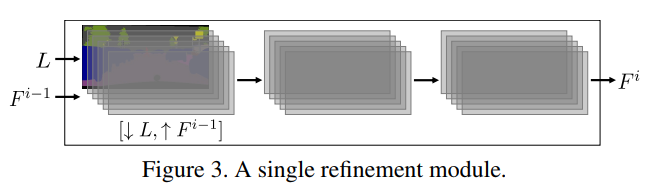
Each module $M^i$ consists of 3 feature layers:
Each layer is followed by $3 \times 3$ convolutions, layer normalization, LReLU nonlinearity.

input layer
dimensionality $ w_i \times h_i \times (d_{i-1} + c)$. $d_{i-1}$ 来自bilinearly upsampled feature layer $F^{i-1}$ ，c来自semantic layout L。
intermediate layer
dimensionality $w_i \times h_i \times d_i$ .
output layer
dimensionality $w_i \times h_i \times d_i$

最后一个module的output layer不需要normalization和nonlinearity，而是用linear projection ( $1 \times 1$ convolution), applied to map $F^{\bar i}$ (dimensionality $w_{\bar i} \times h_{\bar i} \times d_{\bar i}$ ) to the output color image (dimensionality $w_{\bar i} \times h_{\bar i} \times 3$ )。

The total number of refinement modules in a cascade depends on the output resolution.

Cityscape dataset例子中，9个Module，resolution从4x8到1024x2048.对于 $d_i$ ， $i = 0..4$ 为1024， $i = 5,6$ 为512， $i = 7$ 为128， $i = 8$ 为32。

Training

supervised, semantic segmentation dataset $\mathcal D = \{ (I, L) \}$ .
input is semantic layout L, output is corresponding color image I.

loss function (critical, as problem is constrained)
只逐个比较像素值是绝对不够的。而是采用了Gatys et al.提出的content representation或者叫做perceptual loss或feature matching的方法。
The basic idea is to match activations in a visual perception network that is applied to the synthesized image and separately to the reference image. 就是合成图和真实图同时放一个visual perception network里跑，比较(每层的)输出。

$\Phi$ , trained visual perception network (此例是VGG-19). Layers in the network represent an image at increasing levels of abstraction: from edges and colors to objects and categories. Matching both lower-layer and higher-layer activations in the perception network guides the synthesis network to learn both fine-grained details and more global part arrangement.
$\{\Phi_l\}$ , collection of layers in the network $\Phi$ . Each layer is a three-dimensional tensor.

For a training pair $(I, L) \in \mathcal D$ , loss is:

$\mathcal L_{I, L}(\theta) = \sum_l \lambda_l \parallel {\Phi_l(I) - \Phi_l(g(L; \theta ))} \parallel_1$

$g$ is the image synthesis network being trained, $\theta$ is the set of parameters of this network. hyperparameters $\{\lambda_l \}$ balance the contribution of each layer $l$ to the loss.

For layers $\Phi_l (l \ge 1)$ we use ‘conv1_2’, ‘conv2_2’, ‘conv3_2’, ‘conv4_2’, ‘conv5_2’ in VGG-19.
Hyperparameters $\{\lambda_l \}$ are initialized to the inverse of the number of elements in each layer.

Synthesizing a diverse collection

同一个semantic layout理论上能生成多个synthesized image。
所以修改loss function, that encourages diversity within the collection, to emit a collection of images in one shot.

改动：

output channels
3k <- 3, k is the desired number of images. 连续3个channel组成一张图。
loss
用这k个图片的best synthesized image的loss。
$g_u(L;\theta)$ , the $u^{th}$ image in the synthesized collection.
$ min_u \sum_l \lambda_l \parallel {\Phi_l(I) - \Phi_l(g_u(L; \theta ))} \parallel_1 $
loss进阶
这k个图片每个semantic class的最佳表现之和作为loss。This loss in effect constructs a virtual image by adaptively taking the best synthesized content for each semantic class from the whole collection, and scoring the collection based on this assembled image.
拿出VGG-19中每个被比较的layer如conv5_2的每个feature map(CNN的layer有depth)，用 $L_p^l$ 取模只拿出此semantic class的误差值，求和加起来，然后取出最小值，就是这个semantic class的最优结果。以此类推，拿出所有class的最优结果后求和。
前文提到semantic layout有 $c$ 个class。对于input label map中的semantic class $p$ ，用 $L_p$ 来表示 $L(\cdot, \cdot, p)$ .
$\sum_{p=1}^c min_u \sum_l \lambda_l \sum_j \parallel {L_p^l \circ (\Phi_l^j (I) - \Phi_l^j (g_u(L; \theta ))) } \parallel_1 \Phi_l^{j$表示$\Phi_l$的$j}{th}$ feature map.
$L_p^l$ 作为mask使用， $L_p$ downsampled to match the resolution of $\Phi_l$ .
$\circ$ 是Hadamard product，其实就是两个同样dimension的矩阵，相同位置的两个元素相乘。

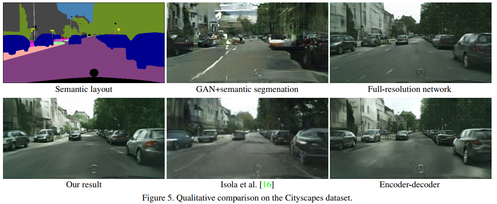
Results

作者尝试的其他方法、前人成果与本方法的比较。
Image Loading

Code

原作者放出了源码。

Ref:
1] http://cqf.io/ImageSynthesis/