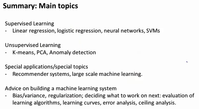
Machine Learning 课程笔记

Coursera上的机器学习公开课，据说是实际授课的弱化版本。

---

Introduction

Welcome

Machine Learning

• Grew out of work in AI
• New capability for computers

Examples:

• Database mining
  Large datasets from growth of automation/web.
  E.g., Web click data, medical records, biology, engineering.
• Applications can’t program by hand
  E.g., Autonomous helicopter, handwriting recognition, most of Natural Language Processing(NLP), Computer Vision.
• Self-customizing programs
  E.g., Amazon, Netflix product recommendations.
• Understanding human learning(brain, real AI).

What is machine learning

Machine Learning definition

• Arthur Samuel(1959). Machine Learning: Field of study that gives computers the ability to learn without being explicitly programmed.
• Tom Mitchell(1998) Well-posed Learning Problem: A computer program is said to learn from experience E with respect to some task T and some performance measure P, if its performance on T, as measured by P, improves with experience E.

Machine learning algorithms:

• Supervised learning
• Unsupervised learning

Others: Reinforcement learning, recommender systems.
Also talk about: Practical advice for applying learning algorithms.

Supervised Learning

“right answers” given.

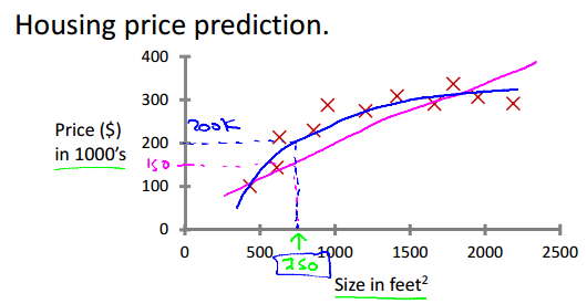
Regression: Predict continuous valued output.(E.g. Housing price prediction.)

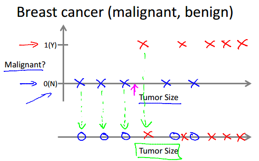
Classification: Discrete valued output(0 or 1).(E.g. Breast cancer(malignant, benign).)

Unsupervised Learning

E.g., Related news, Genes, Organize computing clusters, Social network analysis, Market segmentation, Astronomical data analysis, Cocktail party problem(分辨混合音源中的不同声音).

---

Linear Regression with One Variable

Model representation

Supervised Learning: Given the “right answer” for each example in the data.
Regression Problem: Predict real-valued output.

Notation:
m = Number of training examples
x’s = “input” variable / features
y’s = “output” variable / “target” variable

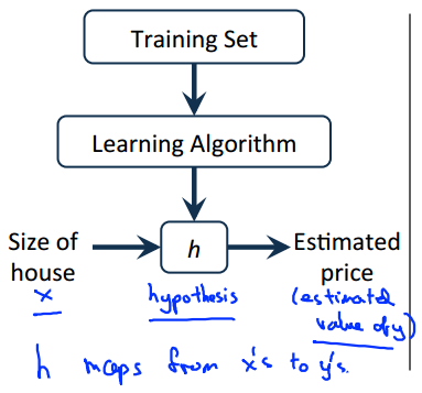
Cost function

Hypothesis: $h_{\Theta}(x)={\Theta}_0+{\Theta}_1x$
${\Theta}_i$'s: Parameters

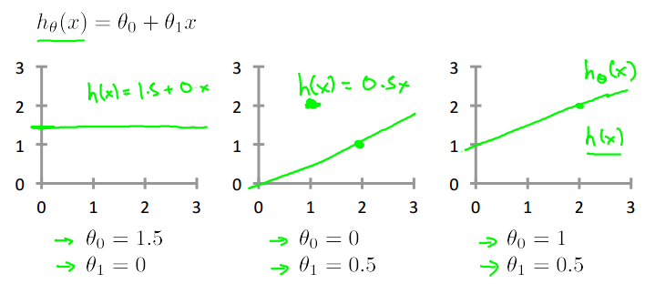
Idea:
Choose $\Theta0$, $\Theta1$ so that $h_{\Theta}(x)$ is close to $y$ for our training examples $(x,y)$.

Cost function intuition

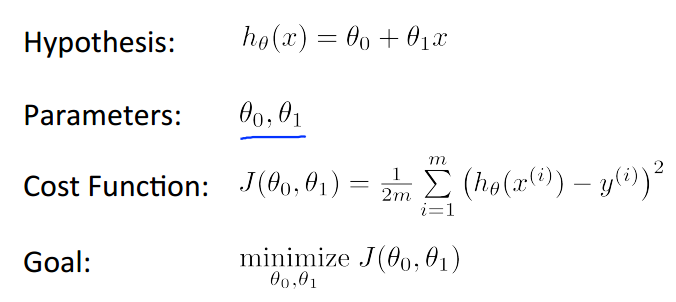
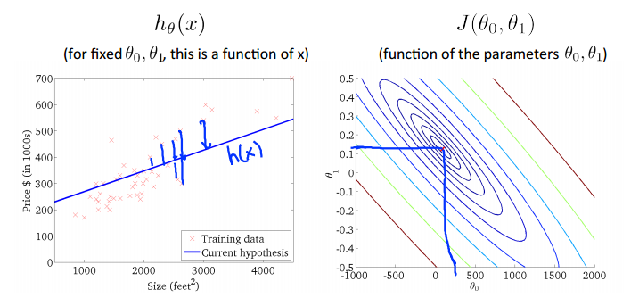
用很多不同的两值计算出误差，画一张误差表，可以看出走势图。

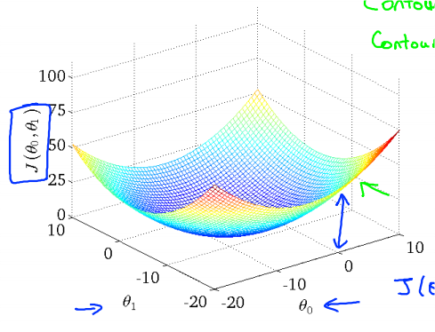
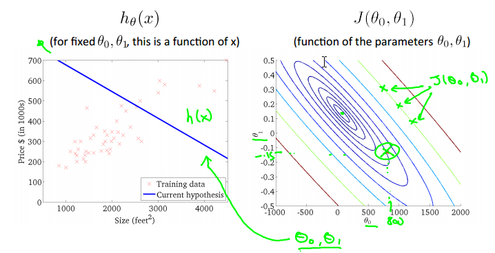
可以用Contour figure来表示。同一条曲线上误差值相同。

Gradient descent

Have some function $J({\Theta}_0,{\Theta}_1)$

Want ${min}_{ {\Theta}_0,{\Theta}_1 } J({\Theta}_0,{\Theta}_1)$

Outline:

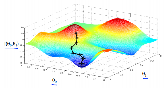
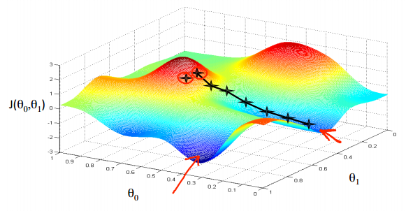
• Start with some ${\Theta}_0, {\Theta}_1$
• Keep changing ${\Theta}_0,{\Theta}_1$ to reduce $J({\Theta}_0,{\Theta}_1)$ until we hopefully end up at a minimum

起点稍有不一样就可能结果不同，有Local optima问题。

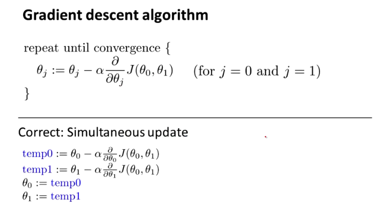
Algorithm:
每个参数单独一点点聚合。
$\alpha$表示Learning rate，是一个调节变量。注意要先同时计算差值，然后再同时更新参数。

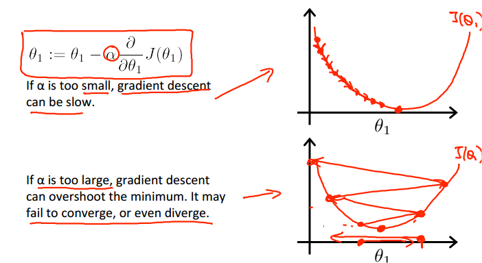
Gradient descent can converge to a local minimum, even with the learning rate $\alpha$ fixed.因为随着误差减小，即使$\alpha$固定，每次调整的数量也会变小。
As we approach a local minimum, gradient descent will automatically take smaller steps. So, no need to decrease $\alpha$ over time.

Gradient descent for linear regression

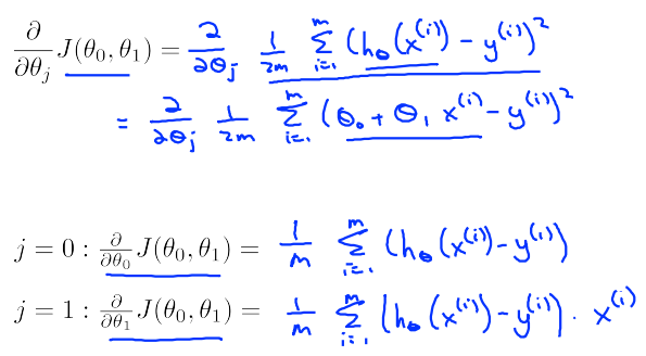
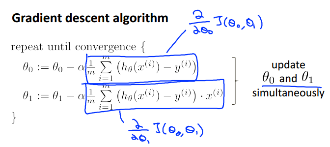
“Batch” Gradient Descent: Each step of gradient descent uses all the training examples.

---

Linear Regression with Multiple Variables

Multiple features

之前X只有一个维度，现在考虑X有多维的情况。

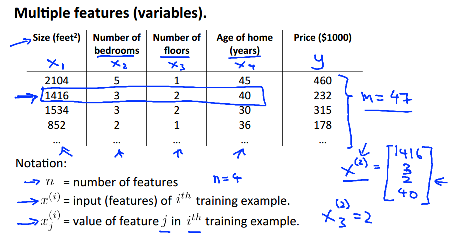
也称作Multivariate linear regression。

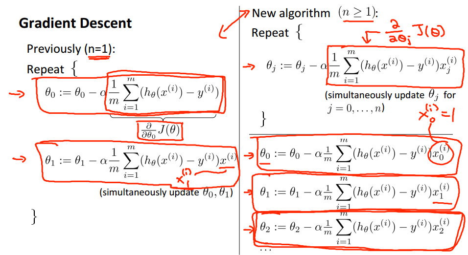
Gradient descent for multiple variables

(注意以下公式的vectorize。有利计算，要多尝试把这些都看做向量、矩阵来计算。)

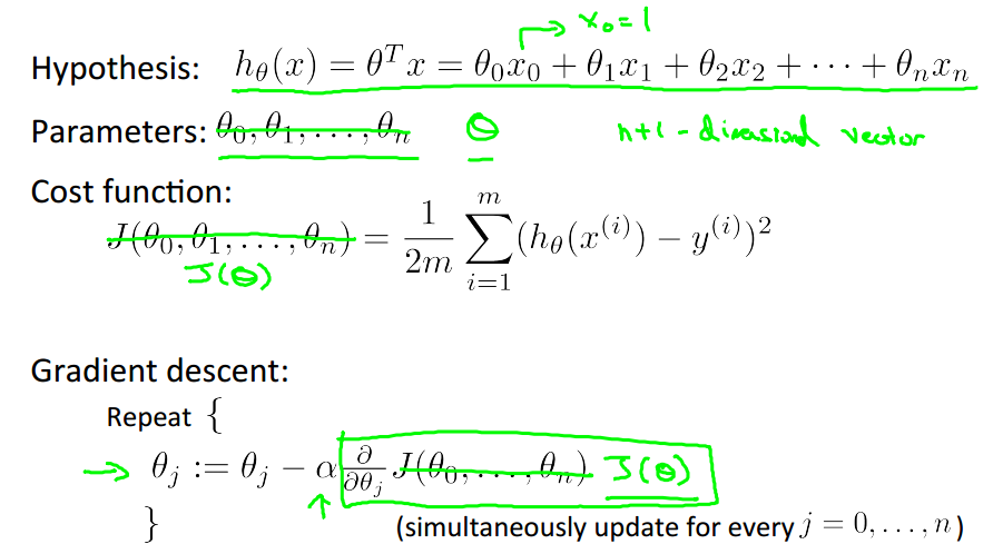
一维只是多维的一个特例。

Gradient descent in practice I: Feature Scaling

Feature Scaling: Get every feature into approximately a $-1 \leqslant x_i \leqslant 1$ range.
E.g. :
原来的取值范围，画出来的J的Coutour figure会是一个拉的很长的细长形状，converge的时候会花费很多时间才能走到中心minimum。
$x_1 = size(0-2000 {feet}^2)$ 和 $x_2 = number of bedrooms(1-5)$
将取值均一化。
x_1 = \cfrac{size({feet}^2)}{2000} 和 x_2 = \cfrac{number of bedrooms}{5}

Mean normalization: Replace $x_i$ with $x_i- {\mu}_i$ to make features have approximately zero mean (Do not apply to $x_0=1$).
E.g.:
x_1= \cfrac{size-1000}{2000} 范围变为 $-0.5 \leqslant x_1 \leqslant 0.5$。
x_2= \cfrac{bedrooms-2}{5} 范围变为 $-0.5 \leqslant x_2 \leqslant 0.5$。

Gradient descent in practice II: Learning rate

Debugging: Making sure gradient descent is working correctly.
确定每次迭代$J(\theta)$都是变小的。当$J(\theta)$小于某个值比如$10^{-3}$时停止迭代，但是这个值很难把握，一般也可以还是看图说话。

How to choose learning rate $\alpha$.
If $\alpha$ is too small: slow convergence.
If $\alpha$ is too large: $J(\theta)$ may not decrease on every iteration; may not converge. (Slow converge also possible.)
Too choose $\alpha$, try: …, 0.001, 0.003, 0.01, 0.03, 0.1, 0.3, 1, …

Features and polynomial regression

多项式回归
对于房子的价格来说，可能有多项影响因素，如长、宽等。
从图中看到，size和price的关系并不是线性关系，如果是二次方的关系曲线末端会变为下降也不太可能，所以可能是三次方的关系。

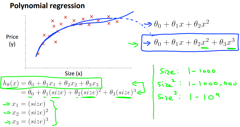
而${size}^3$的取值范围与$size$的取值范围相差太大了，不是最好的选择。这时我们想到，可以用开根号。
于是可以$h_{\theta}(x)={\theta}_0+{\theta}_1(size)+{\theta}_2 \sqrt{(size)}$

Normal equation

除了用Gradient Descent逐步聚合求结果的方法，还有一种用数学公式求解$\theta$的方法。
Normal equation: Method to solve for $\theta$ analytically.
由于目的是求使$J(\theta)$最小的$\theta$值，所以在该处$J(\theta)$的斜率、微分是0，可以据此求解。

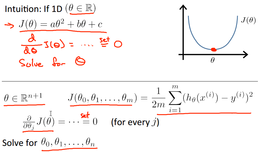
示例：

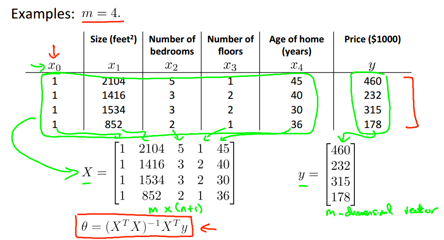
公式就是：$\theta = {(X^TX)}^{-1}X^Ty$
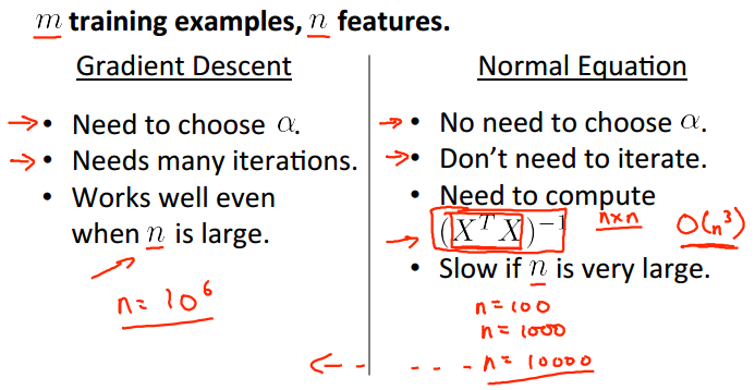
在Octave中的写法是pinv(X'*X)*X'*y。

与Gradient Descent做比较：

Normal equation and non-invertibility

如果$(X^TX)$是不可逆的(singular/degenerate)，在Octave中使用pinv(X'*X)*X'*y仍然可以求出来。
但这时我们最好检查一下自己的数据。可能的原因有：

• Redundant features (linearly dependent). 如x1是size在平方英尺下的值，x2是size在平方米下的值。
• Too many features. 比如$m \leqslant n$，此时应该删除一些feature，或者使用regularization。

---

Logistic Regression

Classification

例子：

• Email: Spam / Not Spam?
• Online Transactions: Fraudulent(Yes / No)?
• Tumor: Malignant / Benign?

$y \in \{ 0,1 \}$
0: “Negative Class” (e.g., benign tumor)
1: “Positive Class” (e.g., malignant tumor)

不适合用linear regression解决，应该用Logistic Regression。

Hypothesis Representation

Logistic Regression Model
Want $0 \leqslant h_{\theta}(x) \leqslant 1$

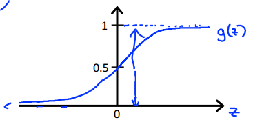
Sigmoid function/Logistic function: h_{\theta}(x) = g({\theta}^Tx) = \cfrac{1}{1+e^{ -{\theta}^Tx} }

它的曲线图类似

Interpretation of Hypothesis Output
$h_{\theta}(x)$ = estimated probability that y=1 on input x

Example:
If $x = \begin{bmatrix} x_0 \\ x_1 \end{bmatrix} = \begin{bmatrix} 1 \\ tumorSize \end{bmatrix}$

$h_{\theta}(x) = 0.7$
Tell patient that 70% chance of tumor being malignant.

"probability that y = 1, given x, parameterized by $\theta$"

$h_{\theta}(x) = P(y=1|x; \theta)$
$P(y=0|x; \theta) = 1 - P(y=0|x; \theta)$

Decision boundary

Logistic regression
$h_{\theta}(x) = g({\theta}^Tx)$ 和 g(z) = \cfrac{1}{1+e^{-z} }。

Suppose predict “y = 1” if $h_{\theta}(x) \geqslant 0.5$。g(z)大于等于0.5，是当z大于等于0时。带入公式，即是当${\theta}^Tx \geqslant 0$时。

同理，predict “y = 0” if $h_{\theta}(x) < 0.5$ 也既是当${\theta}^T x < 0$时。

Decision Boundary

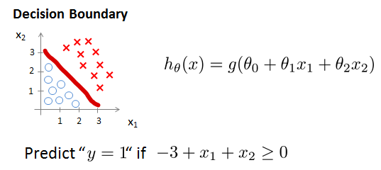
为${\theta}_0, {\theta}_1, {\theta}_2$分别取值-3,1,1。画出$x_1+x_2=3$的图，这就是Decision boundary。

Non-linear decision boundaries

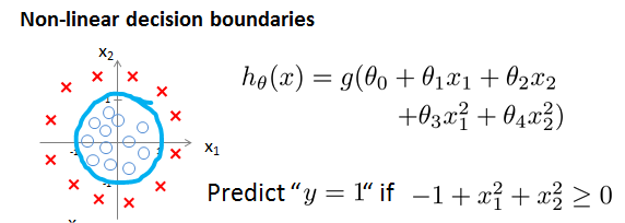
对于复杂一些的公式也是一样，分别取值-1,0,0,1,1。画出曲线图，即是Decisioin boundary。

Cost function

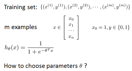
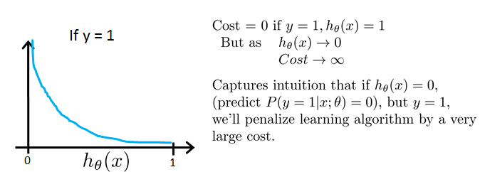
Logistic regression cost function

x轴是$h_{\theta}(x)$，y轴是Cost。

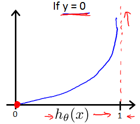
Simplified cost function and gradient descent

Logistic regression cost function

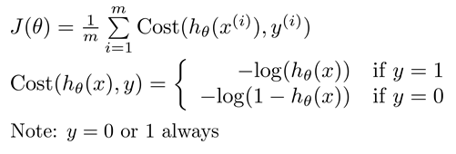
其中的$J(\theta)$作为比较，Linear regression的是这样的：

而Logistic regression的$J(\theta)$可以简化为：

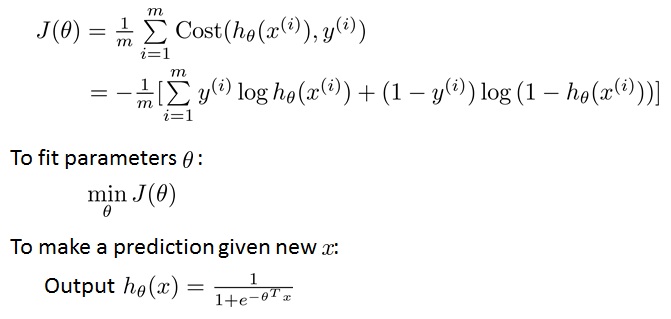
目标就是求得使$J(\theta)$最小的$\theta$。

Gradient Descent

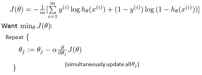
即

Algorithm looks identical to linear regression!

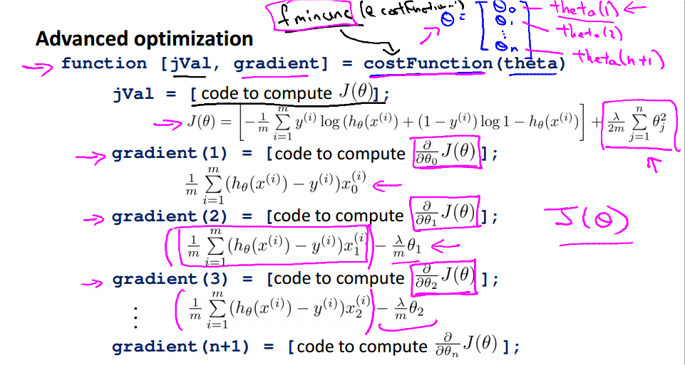
Advanced optimization

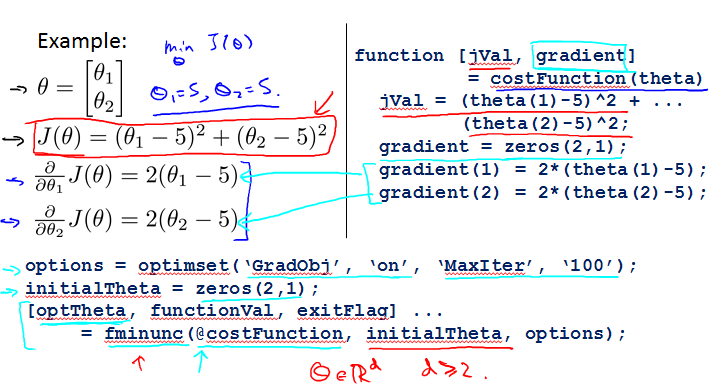
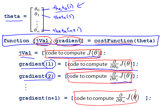
Optimization algorithm

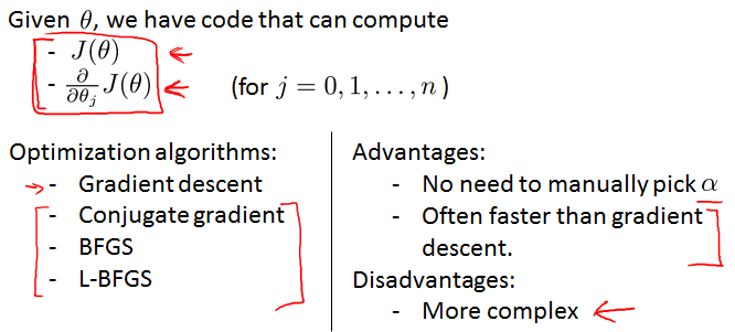
这些高级函数在octave里已有实现。
一个例子，在octave里：

Multi-class classification: One-vs-all

Multiclass classification
Examples:
Email foldering/tagging: Work, Friends, Family, Hobby
Medical diagrams: Not ill, Cold, Flu
Weather: Sunny, Cloudy, Rain, Snow

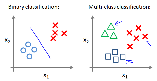
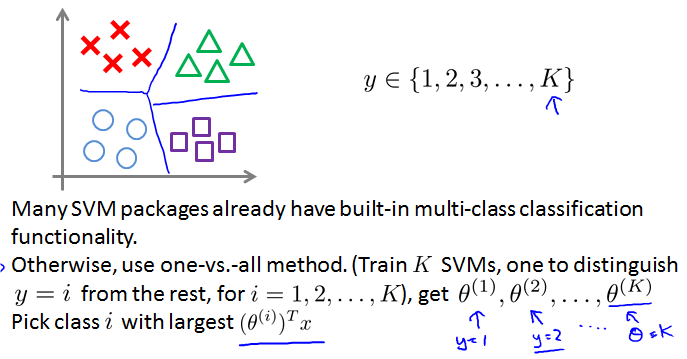
处理多class要用到one-vs-all方法。

One-vs-all (one-vs-rest):
每次针对其中一组和其他组。如下图就分成3个Classifier。

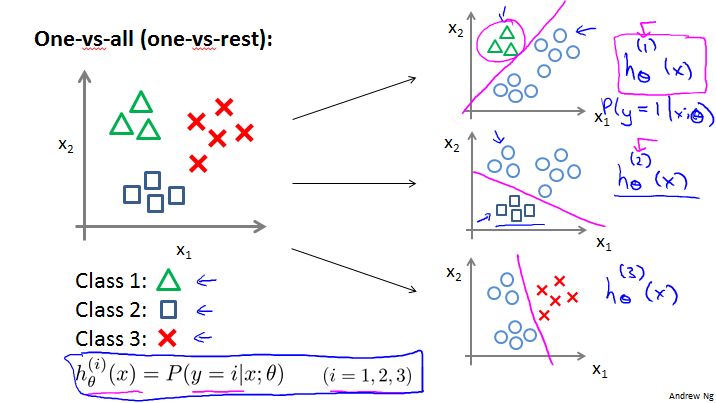
Train a logistic regression classifier $h_{\theta}^{(i)}(x)$ for each class $i$ to predict the probability that $y=i$.

On a new input $x$, to make a prediction, pick the class $i$ that maximazes.

---

Regularization

The problem of overfitting

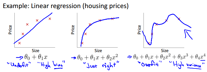
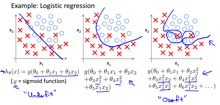
Overfitting: If we have too many features, the learned hypothesis may fit the training set very well ($J(\theta)=0$), but fail to generalize to new examples (predict prices on new examples).

Example: Linear regression (housing prices)

Example: Logistic regression

Addressing overfitting:
如果feature很少，可以画出图。如果feature太多，有两个选择：

1. Reduce number of features.
   Manually select which features to keep.
   Model selection algorithm (later in course).
2. Regularization.
   Keep all the features, but reduce magnitude/values of parameters ${\theta}_j$.
   Works well when we have a lot of features, each of which contributes a bit to predicting $y$.

Cost function

Intuition

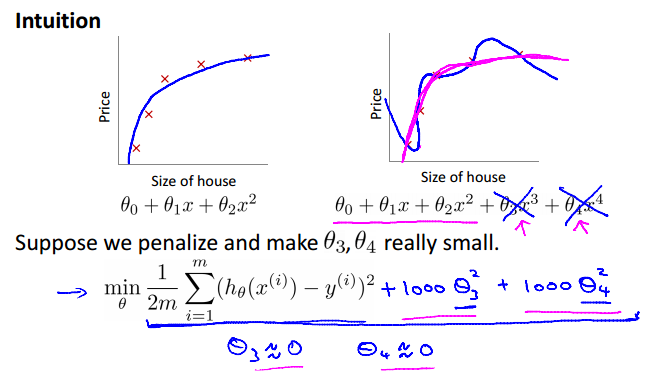
如果想让这个式子的值很小那么${\theta}_3$和${\theta}_4$必须很小。

Regularization
Small values for parameters ${\theta}_0, {\theta}_1, ..., {\theta}_n$

• “Simpler” hypothesis
• Less prone to overfitting

Housing:

• Features: $x_1, x_2, ..., x_{100}$
• Parameters: ${\theta}_0, {\theta}_1, {\theta}_2, ..., {\theta}_100$

由于不知道应该减少哪些$\theta$，所以全部减少。

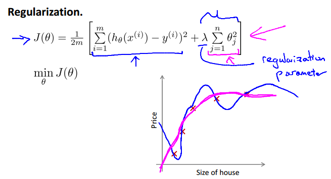
如果$\lambda$特别大，那么从${\theta}_1$到${\theta}_n$几乎都为0，那么$h(\theta)={\theta}_0$，是一条横线。不能消除overfitting，反而导致underfitting。对算法本身的执行没影响。Gradient descent会无法converge。

Regularized linear regression

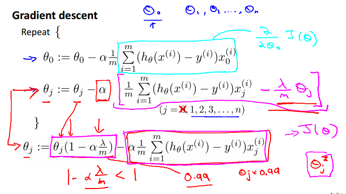
Regularized linear regression

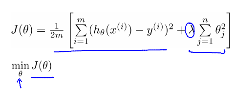
Gradient descent

Normal equation

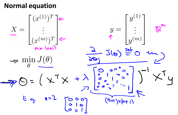
Non-invertibility (optional/advanced)

Regularized logistic regression

Regularized logistic regression

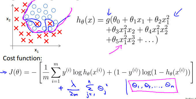
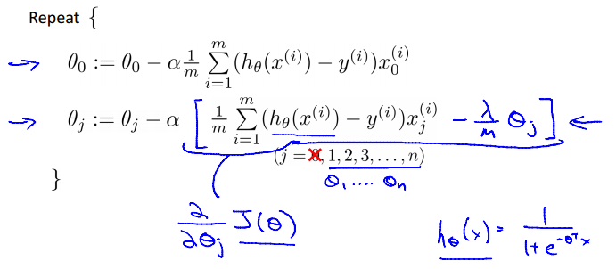
Gradient descent

Advanced optimization

---

Neural Networks Representation

Non-linear hypotheses

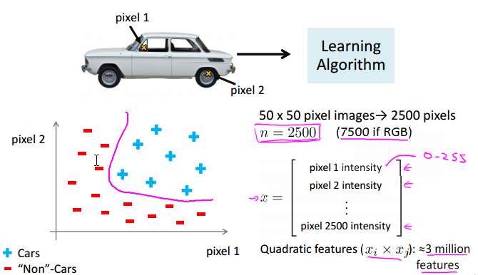
当feature很多的时候，计算起来简直麻烦上天。

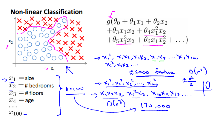
一个Computer Vision例子：


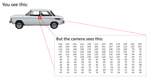
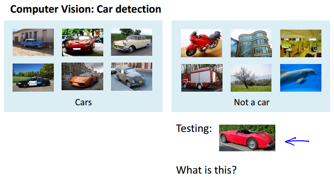
从车的图片和非车的图片固定的地方取两个像素，将其值画在坐标轴上，多次之后可以得到下图左。然而一张图片像素太多了，都以这种方式比较无从计算。

Neurons and the brain

Neural Networks
Origins: Algorithms that try to mimic the brain.
Was very widely used in 80s and early 90s; popularity diminished in late 90s.
Recent resurgence: State-of-the-art technique for many applications.
现在又火起来是因为计算机的计算能力提高了。

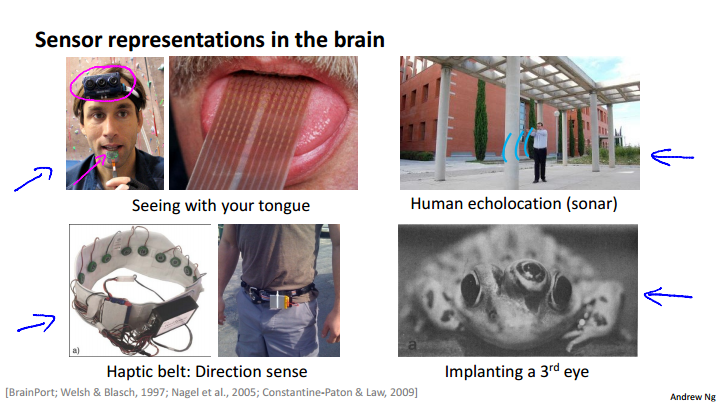
The “one learning algorithm” hypothesis
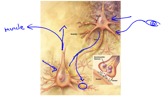
如果切断耳朵与Auditory Cortex之间的神经，把通往眼睛的接上，听觉中枢会学会看。同样，切断手与Somatosensory Cortex之间的神经，把通往眼睛的接上，触觉中枢也会学会看。

Sensor representations in the brain

Model representation

Neuron in the brain

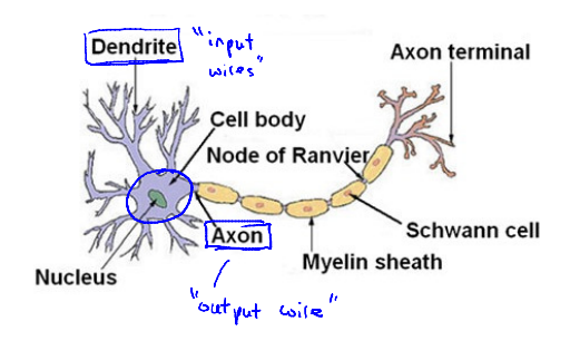
Neuron model: Logistic unit

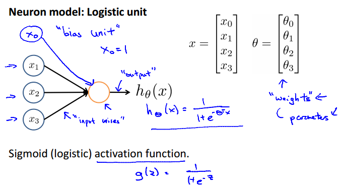
bias unit / input / output / weights = parameters

Neural Network

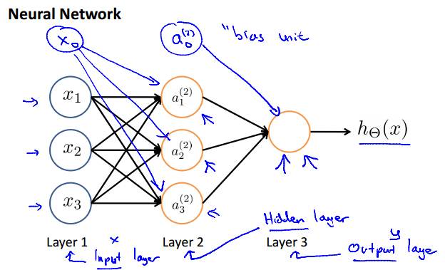
input layer / hidden layer / output layer

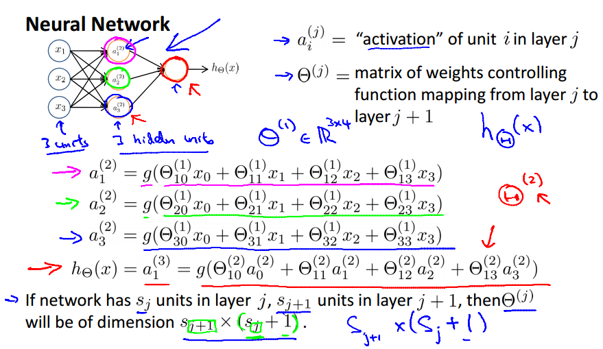
Forward propagation: Vectorized implementation

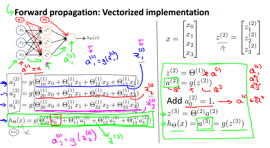
Neural Network learning its own features

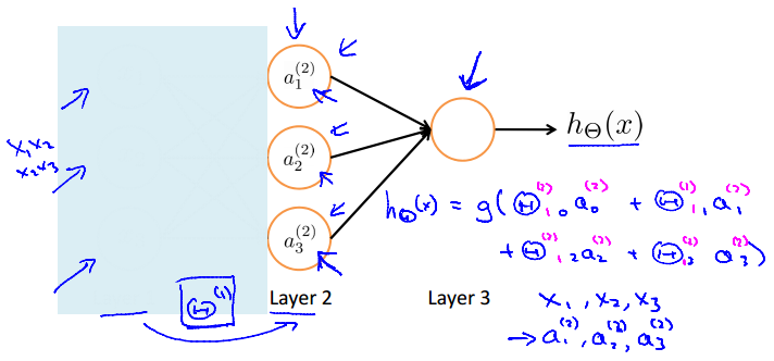
可以看出$h_{\Theta}(x)$与Logistic Regression的很相似，

$h_{\theta}(x)$，只是$\Theta$不同。

Other network architectures

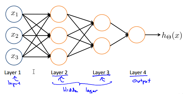
Examples and intuitions

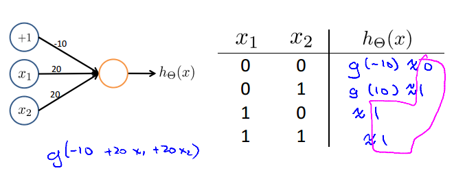
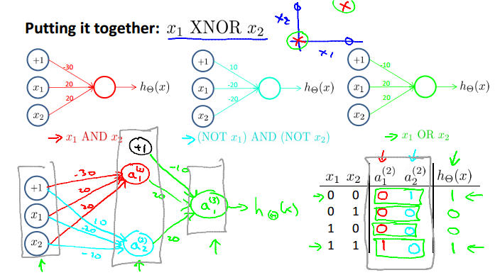
Non-linear classification example: XOR/XNOR

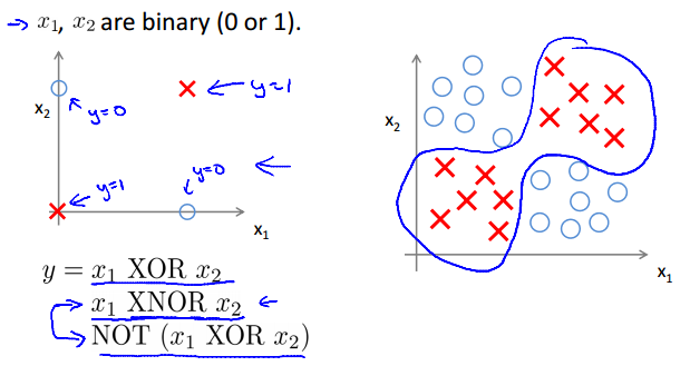
Simple example: AND

Example: OR function

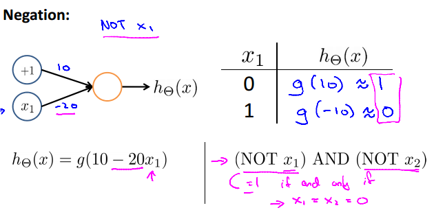
Negation:

Putting it together: $x_1 XNOR x_2$

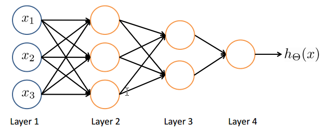
Neural Network intuition

Handwritten digit classification

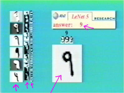
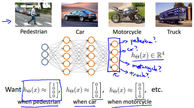
Multi-class classification

Multiple output units: One-vs-all

---

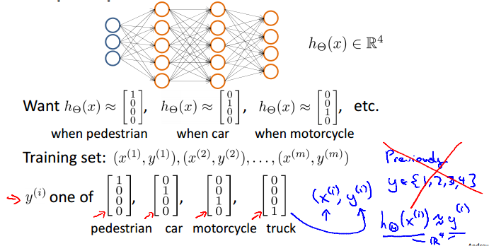
Neural Networks Learning

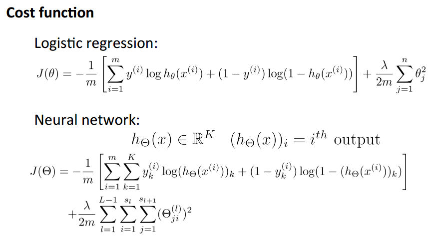
Cost function

Neural Network (Clasification)

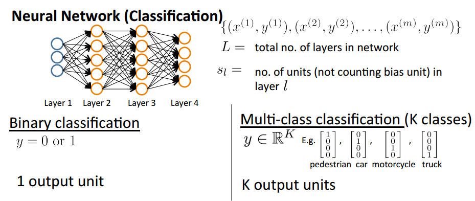
Cost function

Backpropagation algorithm

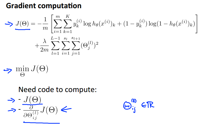
Gradient computation

Gradient computation: Backpropagation algorithm

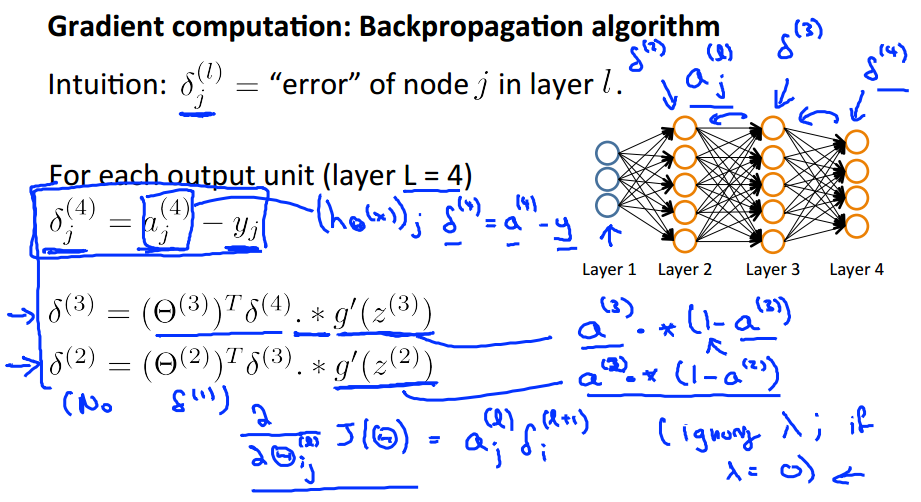
Backpropagation algorithm

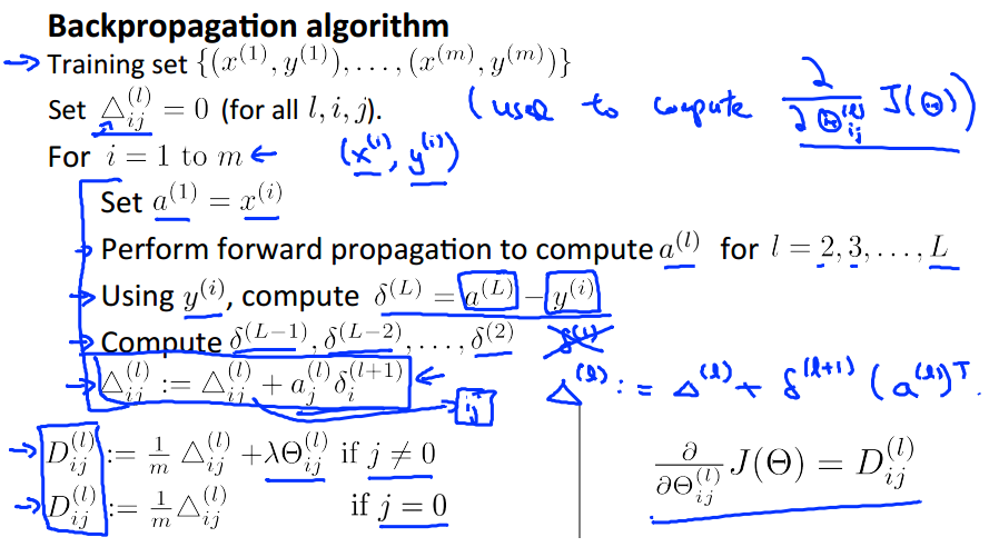
$\Delta$表示全部。

Backpropagation intuition

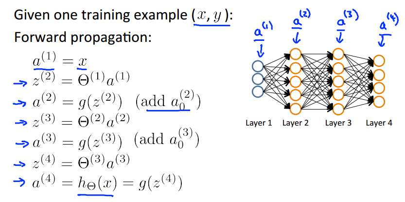
Forward Propagation

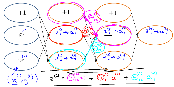
What is backpropagation doing?
简化一下想一下。

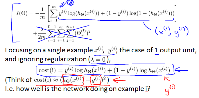
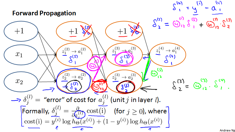
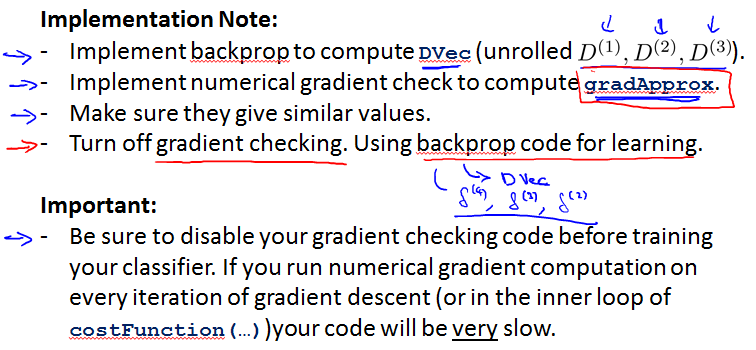
Implementation note: Unrolling parameters

Advanced optimization

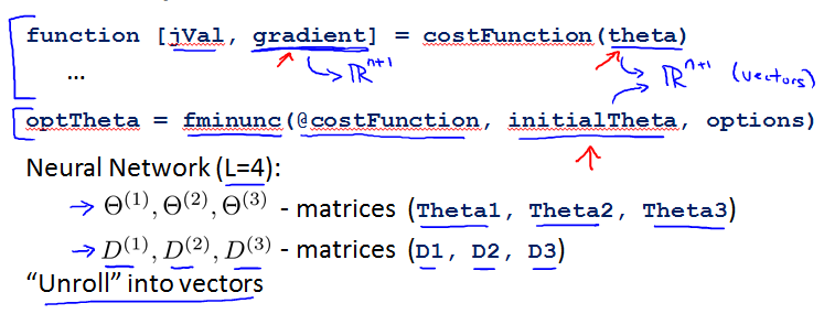
Example

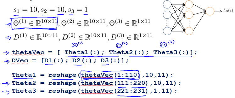
Learning Algorithm

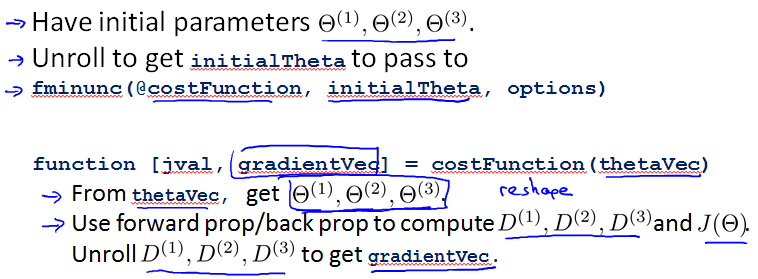
Matrix的好处：forward propagation和back propagation时更方便。
Vector的好处：用advanced optimization algorithms时需要。

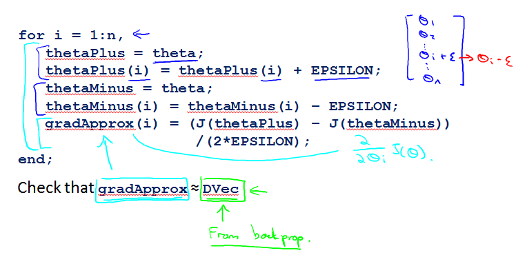
Gradient checking

可以排除几乎所有可能bug。
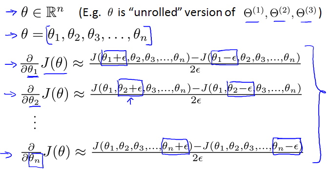
Numerical estimation of gradients
假设$\theta$是实数。

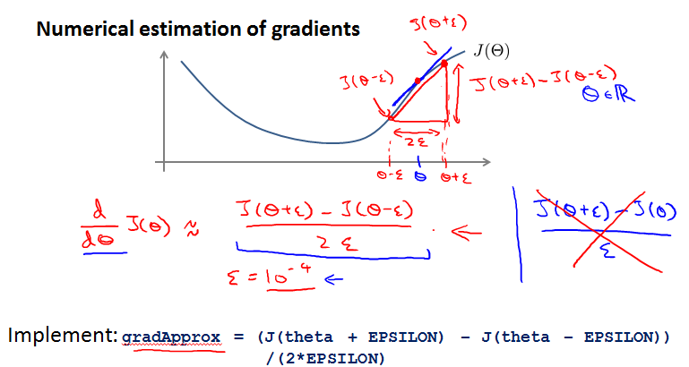
$\varepsilon$的取值也不能太小，运算上可能有numerical problem。通常用${10}^{-4}$。

Parameter vector $\theta$

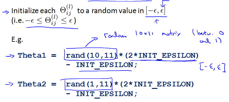
Random initialization

Initial value of $\Theta$
For gradient descent and advanced optimization method, need initial value for $\Theta$.
optTheta = fminunc(@costFunction, initialTheta, options)

Zero initialization

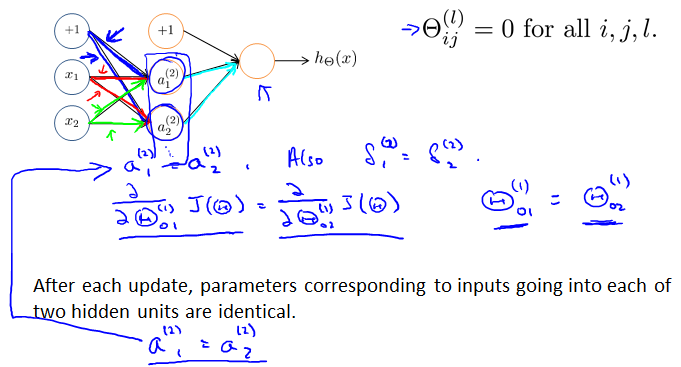
不适用于neural network，会造成每一层里各值都相等，浪费了每层这许多节点。

Random initialization: Symmetry breaking

Putting it together

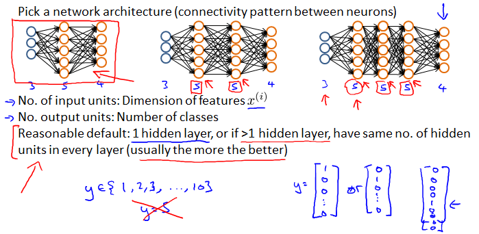
Training a neural network
1.Pick a network architecture (connectivity pattern between neurons)

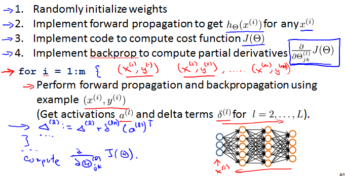
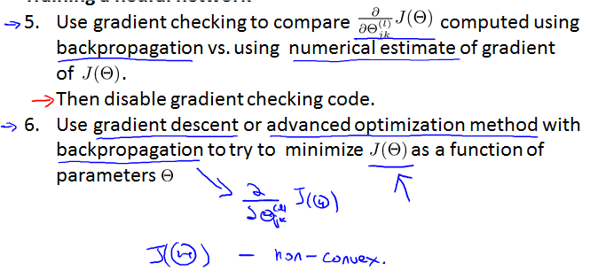
2.Start Training.

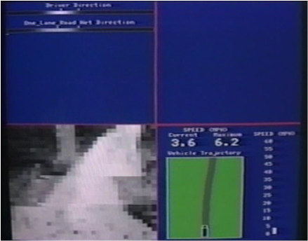
Backpropagation example: Autonomous driving

Dean Pomerleau
左下角是汽车看到的视角。左上第一条是人类司机选择的方向steering direction，第二条是算法选择的方向。

Advice for Applying Machine Learning

Deciding what to try next

Debugging a learning algorithm:

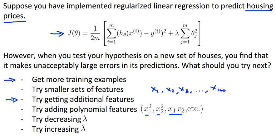
不能盲目尝试下面这些可行策略，应该实现一个Diagnostic。

Machine learning diagnostic:
Diagnostic: A test that you can run to gain insight what is/isn’t working with a learning algorithm, and gain guidance as to how best to improve its performance.
Diagnostics can take time to implement, but doing so can be a very good use of your time.

Evaluating a hypothesis

Evaluating your hypothesis
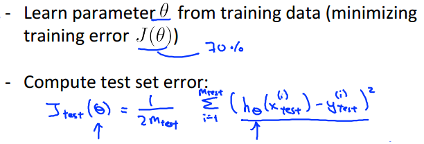
虽然training error很小，然而可能会overfitting。
如果feature很多，又没法plot。此时将数据分成两部分，比例大约7/3，一部分作为Training Set，一部分作为Test Set。（从后面得知这并不是最好的做法，应该三分。）

Training/testing procedure for linear regression

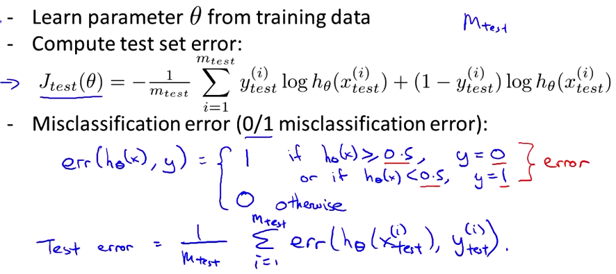
Training/testing procedure for logistic regression

Model selection and training/validation/test sets

Overfitting example
Once parameters ${\theta}_0$, ${\theta}_1$, …, ${\theta}_4$ were fit to some set of data (training set), the error of the parameters as measured on that data (the training error $J(\theta)$ is likely to be lower than the actual generalization error.

Model selection

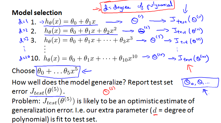
d = degree of polynomial
对每种model进行训练，得到vector $\theta$，然后将其用于test data，得到J，看看哪种model中的J最小。这样的问题是d可能会对test data过拟合，所以得到的错误率过于乐观，并不是很好的做法。

Evaluating your hypothesis

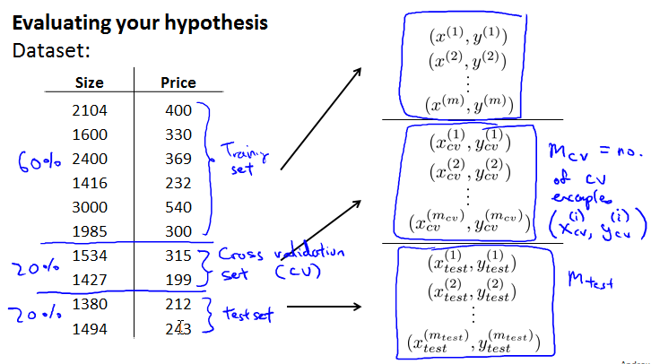
将数据分成三部分，比例大约6/2/2，分别为Training Set/Cross Validation Set/Test Set。
$m_{cv}$表示number of cross validation examples.

Training/validation/test error

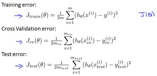
Model selection

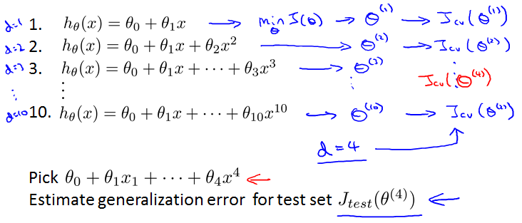
得到$\theta$后在cross validataion set上进行测试，计算J。取其中最小的d。
然后再在test set上运行，计算错误率。

Diagnosing bias vs. variance

不是underfitting就是overfitting。

Bias/variance


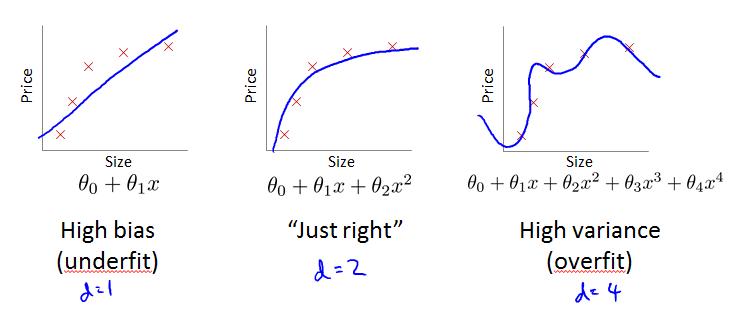
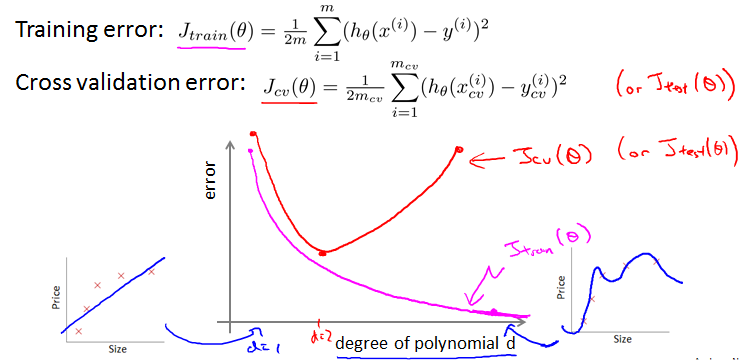
随着d值变大，training error会越来越小，而cross validation error会有一个最小值，从underfitting到overfitting。

Diagnosing bias vs. variance

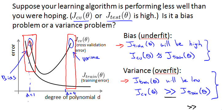
看两者是都高还是一高一低区分under还是over。

Regularization and bias/variance

Linear regression with regularization

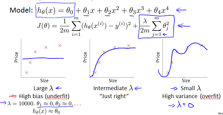
Choosing the regularization parameter $\lambda$

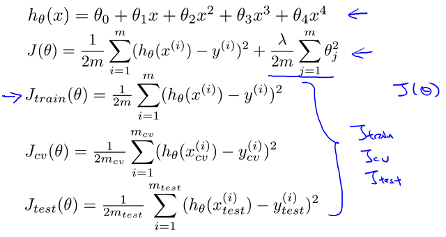
还是分成三组。

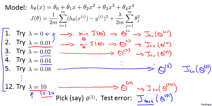
$\lambda$每次乘以2，计算$\theta$，在cross validation组测试计算J，选择最小J的$\lambda$。然后用其在test set里计算test error。

Bias/variance as a function of the regularization parameter $\lambda$

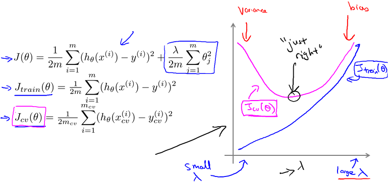
$\lambda$小的时候容易overfitting，大的时候容易underfitting。
实际曲线会noisy一点。

Learning curves

Learning curves

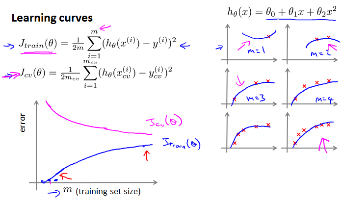
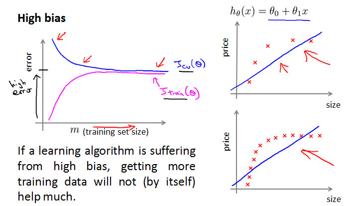
横轴m是training set size。J{train}会逐渐变大，J{cv}会越来越小，这样就对了。

High bias

High variance

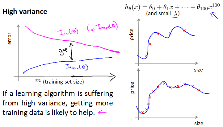
J{train}过小，J{cv}过大，中间有个大gap。并且持续变化，不会平稳。

Deciding what to try next(revisited)

Debugging a learning algorithm

• Get more training examples - fixes high variance，有利于在learning curve中发现问题。
• Try smaller sets of features - fixes high variance.
• Try getting additional features - fixes high bias.
• Try adding polynomial features - fixes high bias.
• Try decreasing $\lambda$ - fixes high bias.
• Try increaing $\lambda$ - fixes high variance.

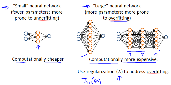
Neural networks and overfitting

Machine Learning System Design

Prioritizing what to work on: Spam classification example

Building a spam classifier
Example.

Supervised learning.

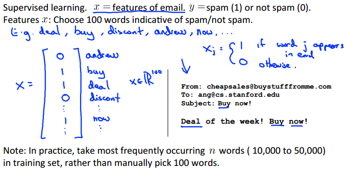
How to spend your time to make it have low error?

• Collect lots of data. E.g. “honeypot” project.
• Develop sophisticated features based on email routing information (from email header).
• Develop sophisticated features for message body, e.g. should “discount” and “discounts” be treated as the same word? How about “deal” and “Dealer”? Features about punctuation?
• Develop sophisticated algorithm to detect misspellings (e.g. m0rtgage, med1cine, w4tches.)

Error analysis

Recommended approach

• Start with a simple algorithm that you can implement quickly. Implement it and test it on your cross-validation data.
• Plot learning curves to decide if more data, more features, etc. are likely to help.
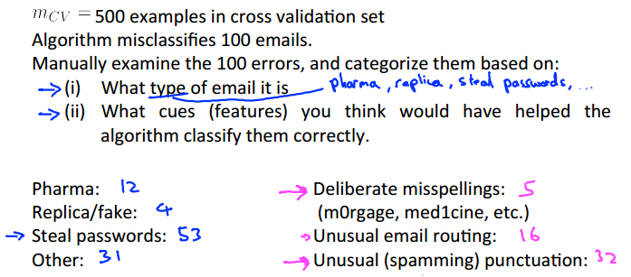
• Error analysis: Manually examine the examples (in cross validation set) that your algorithm made errors on. See if you spot any systematic trend in what type of examples it is making errors on.

Error Analysis

The importantance of numerical evaluation
Should discount/discounts/discouted/discounting be treated as the same word?
Can use “stemming” software (E.g. “Porter stemmer”)
universe/university (不好的情况。)

Error analysis may not be helpful for deciding if this is likely to improve performance. Only solution is to try it and see if it works.
Need numerical evaluation (e.g., cross validation error) of algorithm’s performance with and without stemming.
Without stemming: 5% error
With stemming: 3% error
Distinguish upper vs. lower case(Mom/mom): 3.2%

Error metrics for skewed classes

Cancer classification example

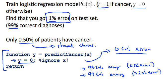
Logistic regression得到1%的错误率。而下面的代码之间全部都改成y=0没cancer反而错误率只有0.5%。
这种两种情况出现比例相差极多的情况就叫skewed classes. More positive examples than negative examples.
用数据衡量这种情况时要用到Precision/Recall。
Precision/Recall

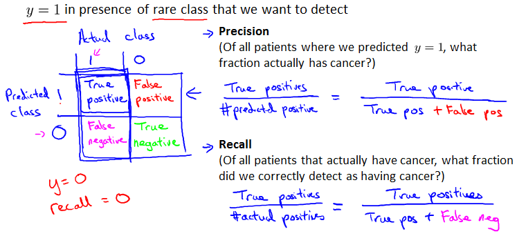
这两值都是越高越好。

Trading off precision and recall

Trading off precision and recall

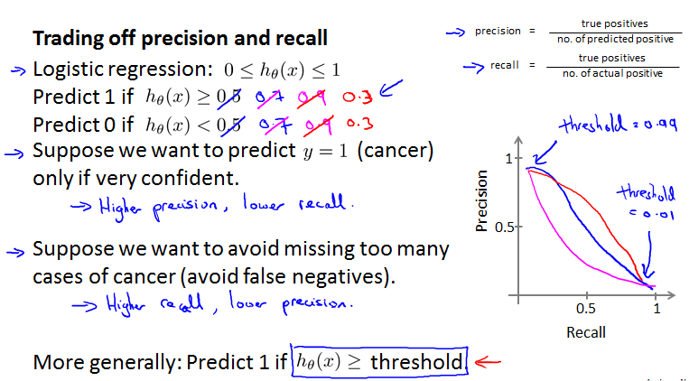
通过修改threshold来操纵precision和recall值来满足自己的要求。
0.9对应第一种情况，0.3对应第二种情况。
曲线可能有多种形状。

$F_1$ Score (F score)

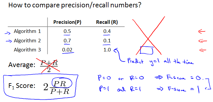
直接求平均不好。还如之前所有直接y=1的情况，recall会很高，影响结果判断。
应该计算$F_1$ Score。相当于将两者的权重都降低了，其中任何一个小，整体都小。

Data for machine learning

Designing a high accuracy learning system

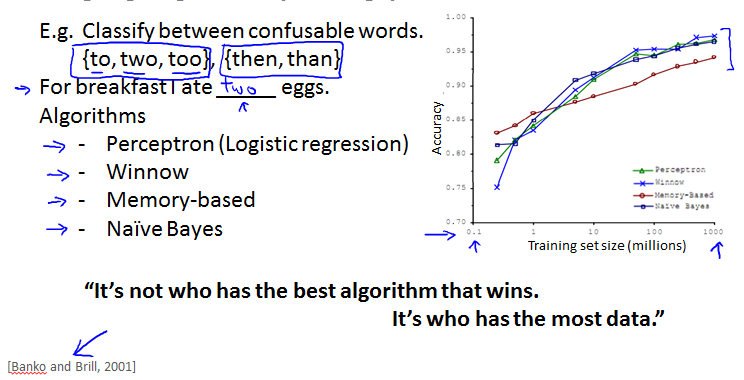
看图得知数据很少时，算法表现差异很大；当数据很多时，它们都差不多了。

Large data rationale

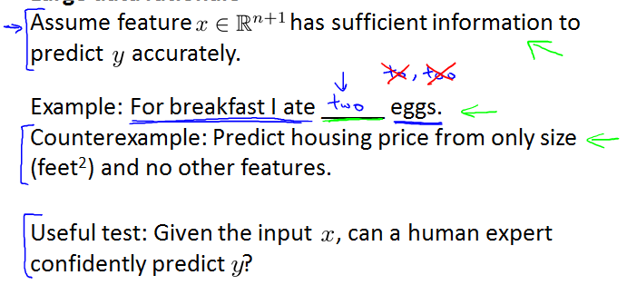
检验上述结论，想想本图的couter example和useful test。

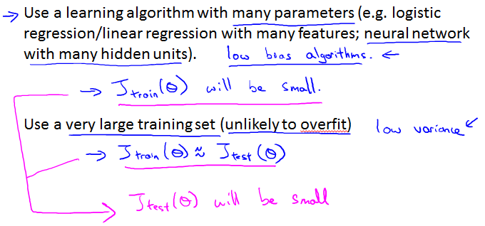
参数多数据多，于是bias和variance都小，结果就是不错。

满足1.人类可以从此数据推断。2.有很多数据。这两点，基本可以确定会有一个好结果。

Support Vector Machines

SVM

Optimization objective

Alternative view of logistic regression


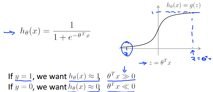
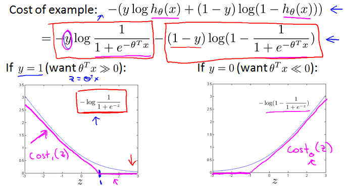
原来的曲线变成多段折线。x轴是z，y轴是cost。

Support vector machine


C可以认为是$1/\lambda$。

SVM hypothesis

Large Margin Intuition

Support Vector Machine

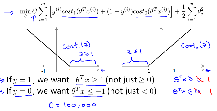
x轴是z，y轴是cost。

SVM Decision Boundary

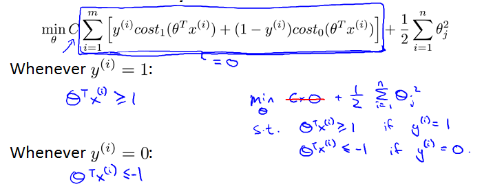
当C特别大时，我们倾向于让框住的那一部分接近0.

SVM Decision Boundary: Linearly separable case

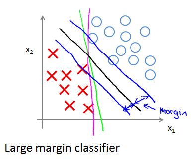
The black decision boundary has a larger distance. That distance is called the margin of the support vector machine. Larger minimum distance from any of the training examples.

Large margin classifier in presence of outliers

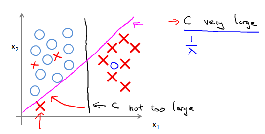
当有outliers时。如果C特别大，会是藕荷色那条线。如果C的值理智一点，就是黑色那条线。C的作用和之前的$\lambda$差不多。

The mathematics behind large margin classification

Vector Inner Product

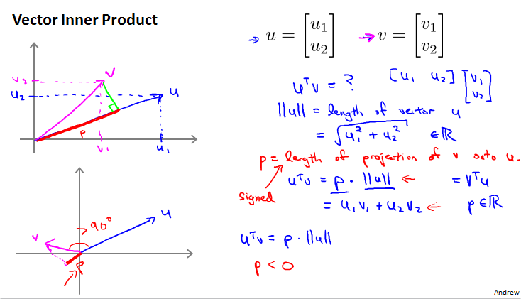
SVM Decision Boundary


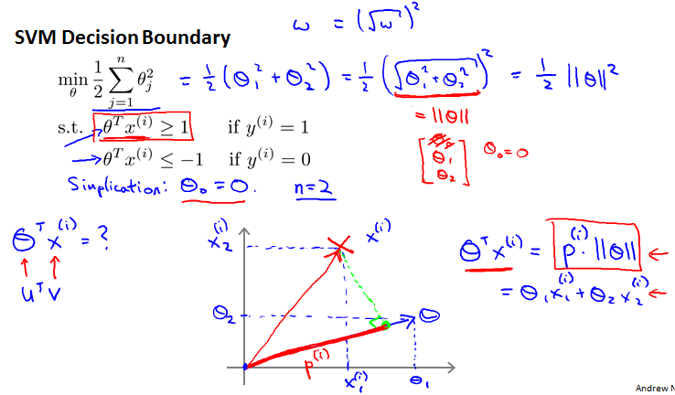
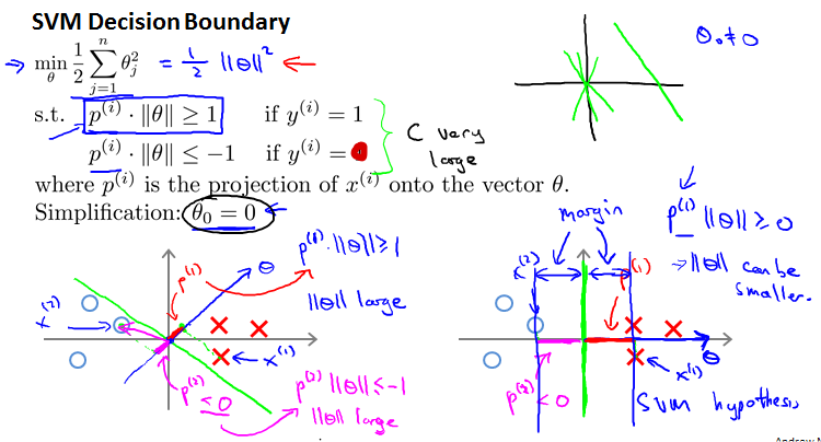
margin就是p。如果不假设${\theta}_0$为0，绿线SVM Decision Boundary就是不过原点。

Kernals

Non-linear Decision Boundary

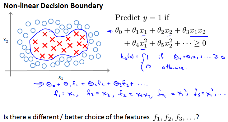
Kernal

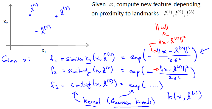
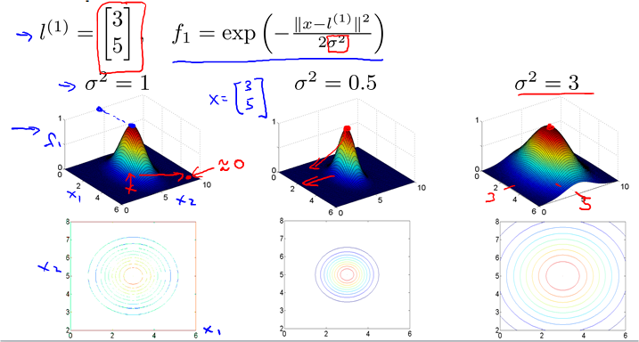
Similarity Functions. Gaussian kernal.

Kernals and Similarity

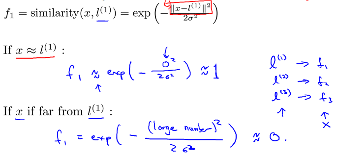
Example


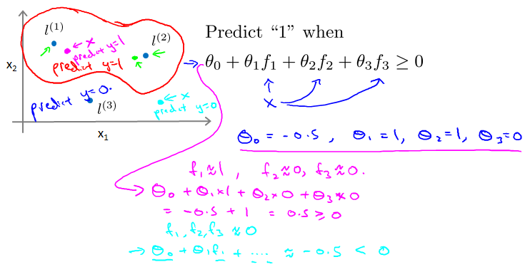
对于藕荷色的点，离l1近，所以f1约等于1；离其他点远，其他f都约等于0。
对于青色的点，都远，所以f都约等于0。
由于Theta3为0，所以boundary就是离l1和l2近的点，如图。

Choosing the landmarks

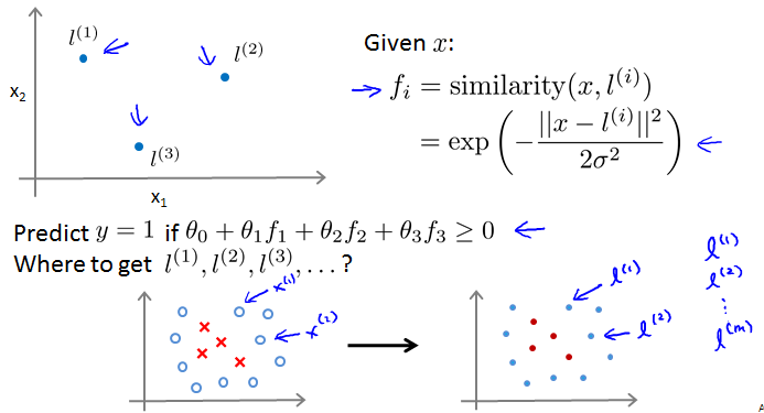
l就是landmarks。就放在training examples上。

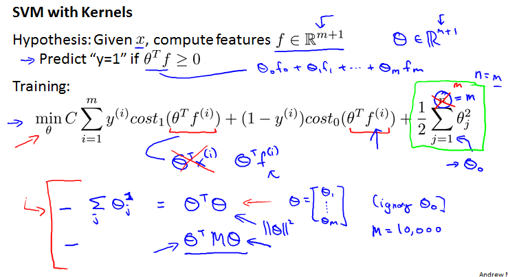
SVM with Kernels

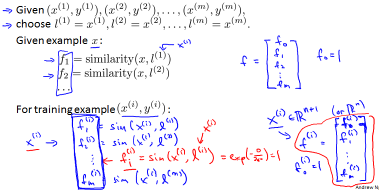
右边的f是feature vector。

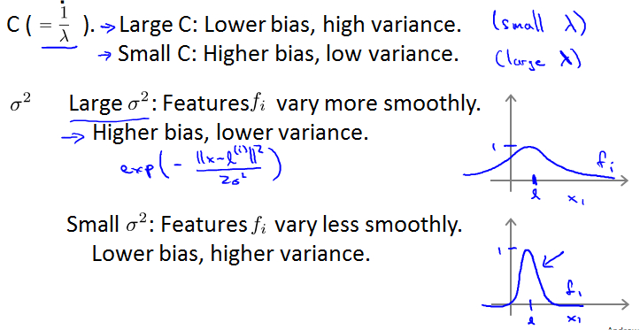
SVM parameters

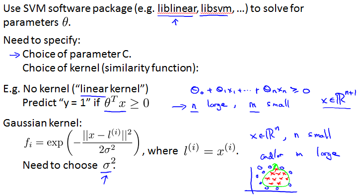
Using an SVM

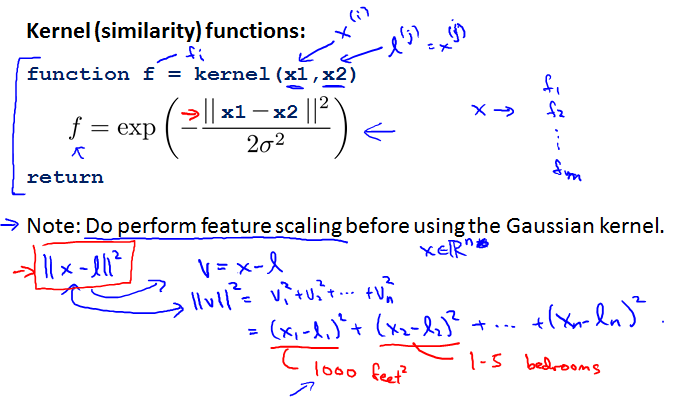
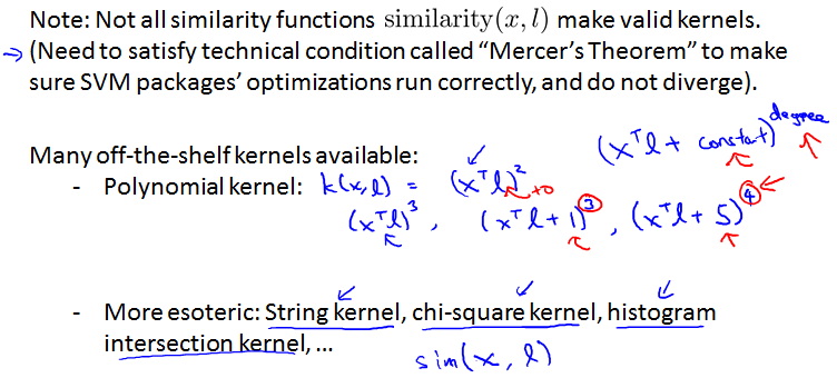
Kernel(similarity) functions:

Other choices of kernel

Multi-class classification

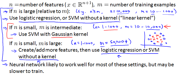
Logistic regression vs. SVMs

Clustering

从这里开始Unsupervised.

Unsupervised learning introduction

Supervised learning

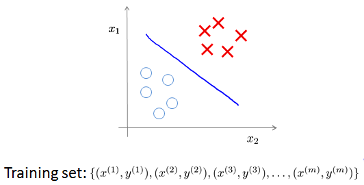
Unsupervised learning

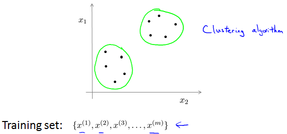
区别是数据有没有label。让algorithm自己找特性。
Applications of clustering

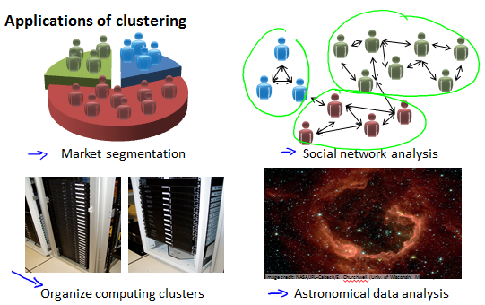
一些clustering算法的应用示例。

K-means algorithm

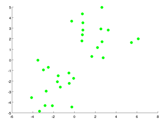
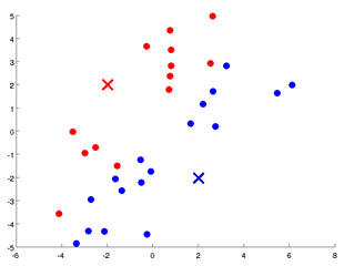
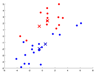
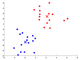
K Means算法是一个重复迭代的算法：

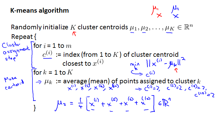
1. cluster assignment step. 将所有点根据所离最近的centroid分组。(最初的centroid是随机的。)
2. move centroid step.将centroid放到自己所在组的中心点。
3. 重复上述两步，直到稳定。

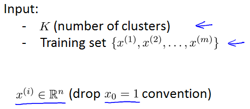
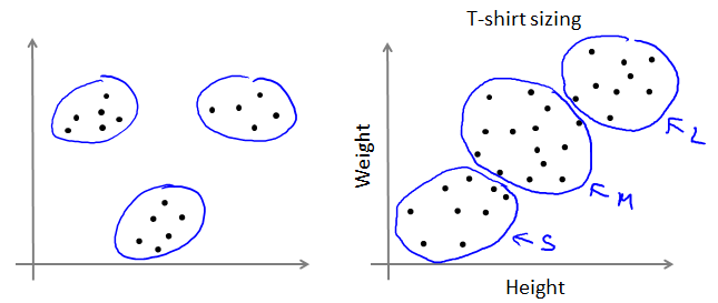
K-means algorithm

K-means for non-separated clusters

Optimization Objective

K-means optimization objective
好处是检查是否正常工作和找到更加cluster和避开local optima。

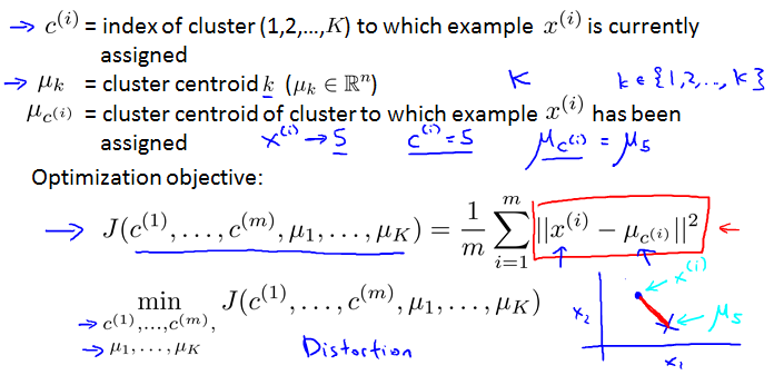
K-means算法的两步就相当于：先固定$\mu$最小化C，再固定C最小化$\mu$。

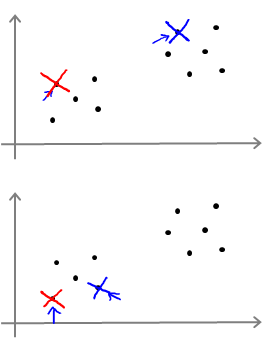
Random initialization

Random initialization
Should have K < m.
Randomly pick K training examples.
Set ${\mu}_1,...,{\mu}_k$ equal to these K examples.
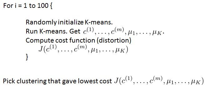
可能效果很好也可能很差。

可能会出现Local optima。

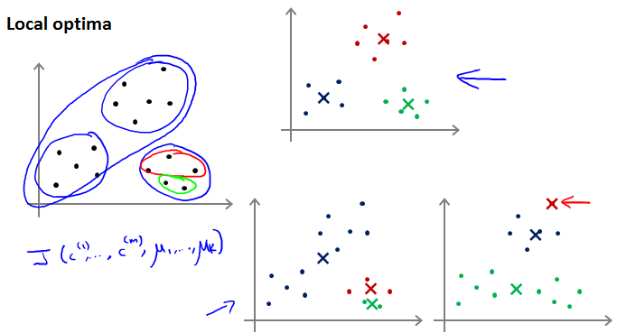
所以应该运行K-means很多次。

Choosing the number of clusters

最常用的还是手动，比如看图。

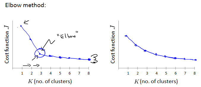
一种方法叫做Elbow method:
用不同的K跑很多遍，计算J，看图，找胳膊肘。有时这个胳膊肘并不明显，如右图。

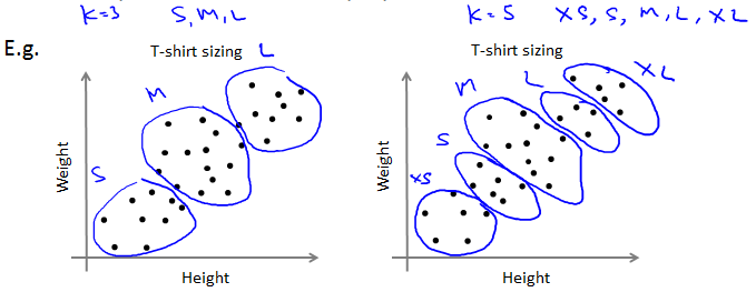
或者K-means的结果之后给别人用，那么就根据之后别人的表现来判断K。
Sometimes, you’re running K-means to get clusters to use for some later/downstream purpose. Evaluate K-means based on a metric for how well it performs for that later porpose.

Dimensionality Reduction

Motivation I: Data Compression

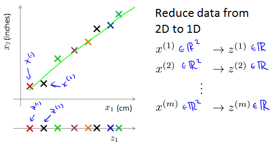
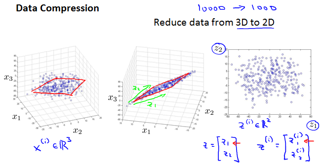
projection.

Motivation II: Data Visualization

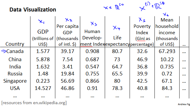
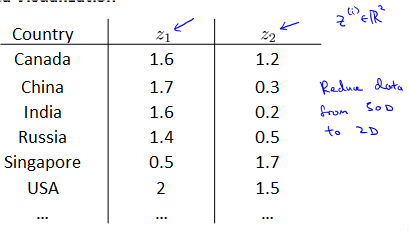
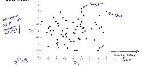
Principal Component Analysis problem formulation

Principal Component Analysis(PCA) problem formulation

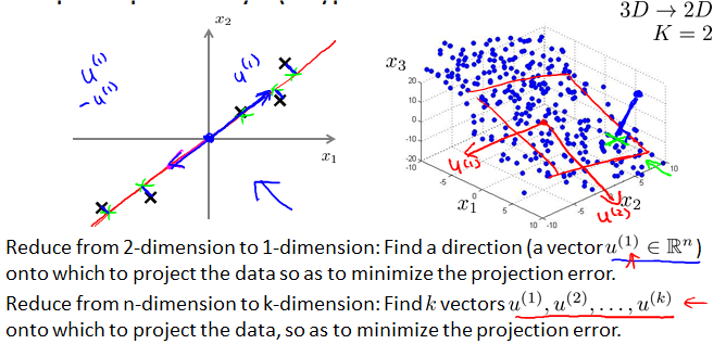
projection error就是从原始位置到投射点的距离。
PCA is not linear regression

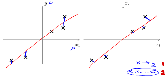
linear regression试图缩小的是点与线之间y方向的距离，因为是要争取让x的表达式最接近y。
PCA试图缩小的是点与线之间的垂直距离，没有y，所有x之间是平等的。

Principal Component Analysis algorithm

Data preprocessing

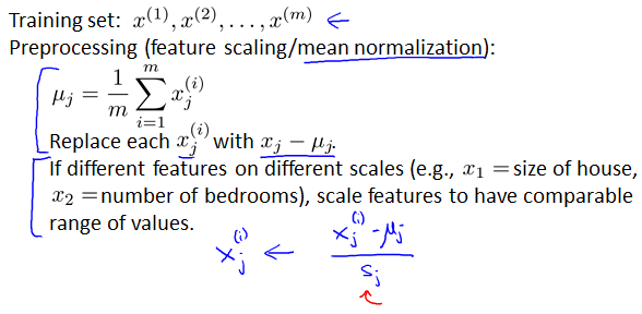
Principal Component Analysis(PCA) algorithm


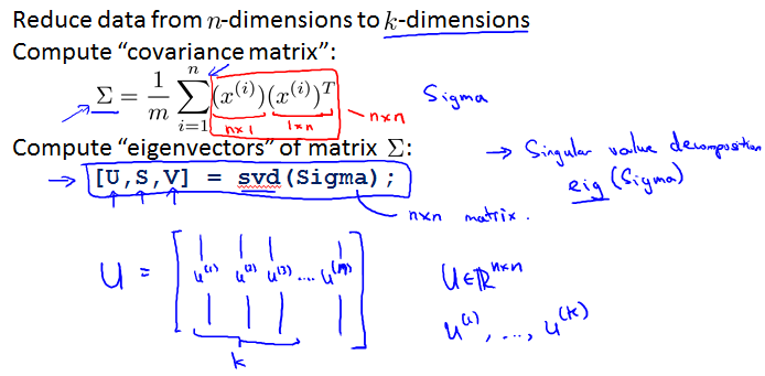
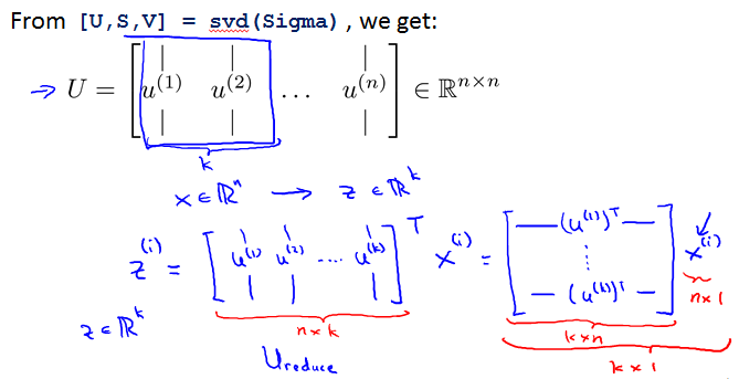
Principal Component Analysis(PCA) algorithm summary

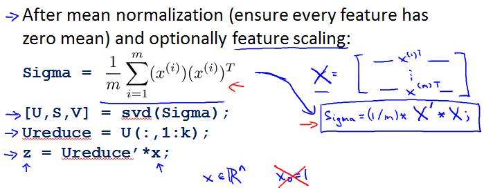
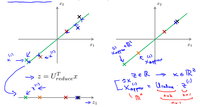
Reconstruction from compressed representation

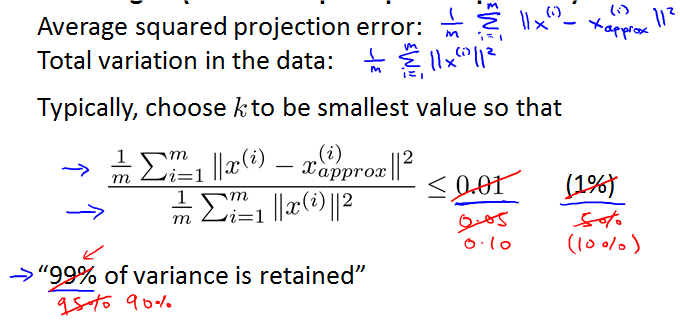
Choosing the Number of Principal Components

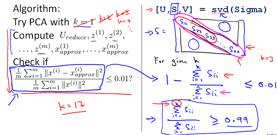
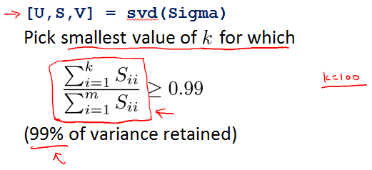
Advice for applying PCA

Supervised learning speedup

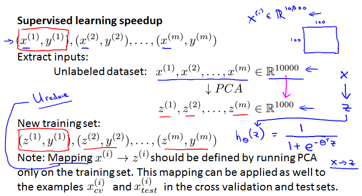
只在training data上运行PCA，计算出$U_{reduce}$后再应用于另两组。

Application of PCA
Compression

• Reduce memory/disk needed to store data.
• Speed up learning algorithm.

Visualization

Bad use of PCA: To prevent overfitting

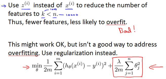
因为PCA还是会损失一些信息。

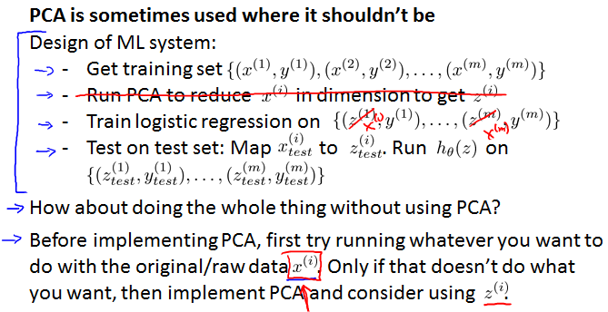
PCA is sometimes used where it shouldn’t be
应该先用原始的进行计算，如果效果不好需要降维才用PCA。

Anomaly Detection

Problem motivation

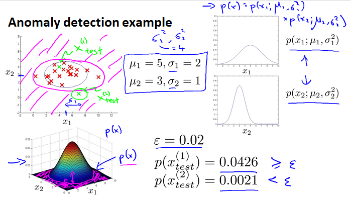
Anomaly detection example



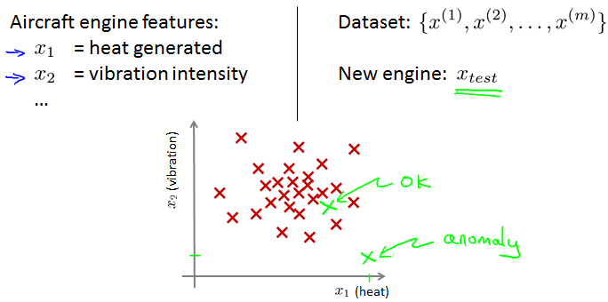
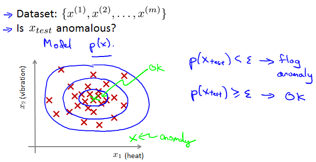
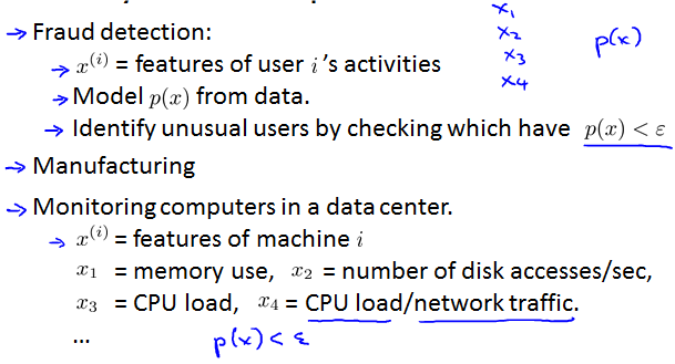
得到feature，建立model，用model计算test数据的数值，看看是否在正常范围内。

Gaussian distribution

Gaussian (Normal) distribution

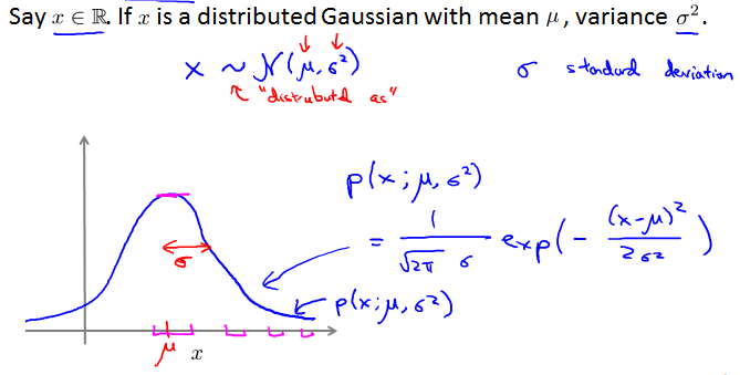
Gaussian distribution example

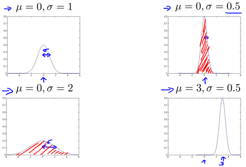
阴影面积总为1。

Parameter extimation

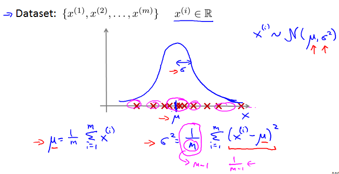
看出数据是经过Gaussian Distribution生成的，计算$\mu$和$\sigma$。

Algorithm

Density estimation

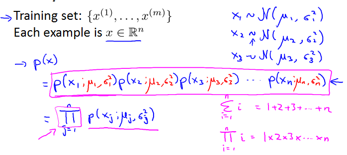
Anomaly detection algorithm

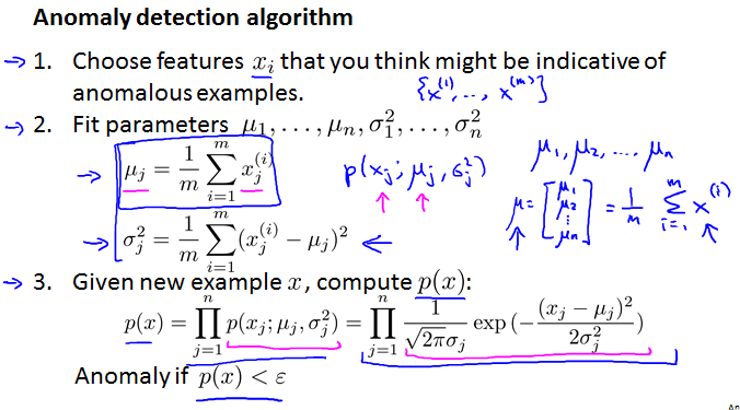
Anomaly detection example

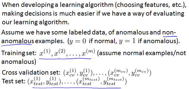
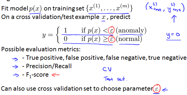
Developing and evaluating an anomaly detection system

The importance of real-number evaluation

Aircraft engines motivating example

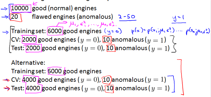
Algorithm evaluation

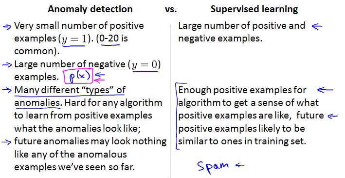
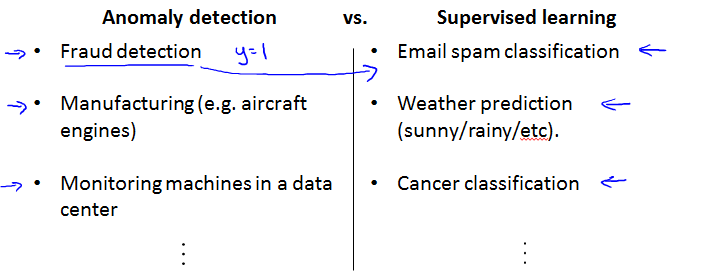
Anomaly detection vs. supervised learning

Choosing what features to use

Non-gaussian features

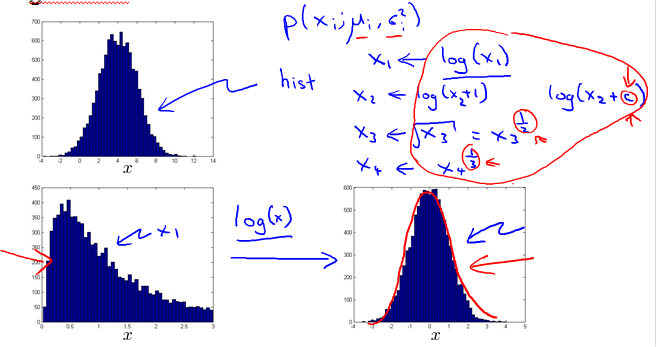
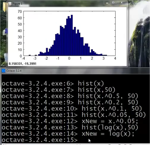
看看直方图像不像Gaussian Distribution。像就可以用。如果不像的话就对数据做一些转换，让它像Gaussian。

Error analysis for anomaly detection

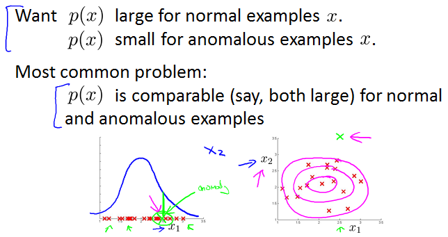
针对这个问题，争取从数据中分析出一个新feature如x2。

Monitoring computers in a data center
Choose features that might take on unusually large or small values in the event of an anomaly. 后两个在有错误时会很大，因为网络负载小时CPU还很忙，一定是有问题了。

• $x_1$ = memory use of computer
• $x_2$ = number of disk accesses/sec
• $x_3$ = CPU load
• $x_4$ = network traffic
• $x_5$ = CPU load / network traffic
• $x_6$ = (CPU load)^2 / network traffic

Multivariate Gaussian distribution

Motivating example: Monitoring machines in a data center

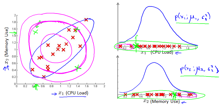
这种情况下，使用传统Gaussian，绿X本该有错，却还在正常范围内。

Multivariate Gaussian(Normal) distributioin

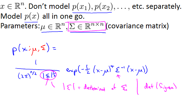
Octave命令det(Sigma)。

Multivariate Gaussian(Normal) examples

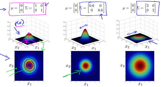
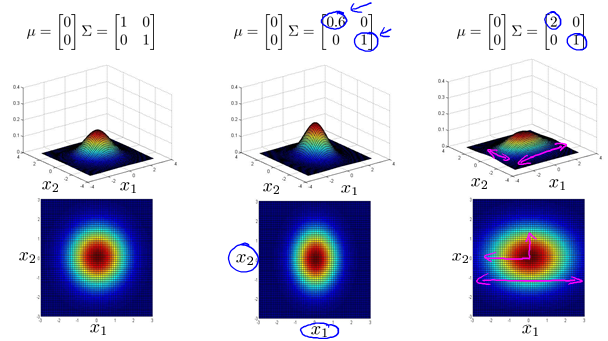
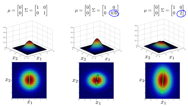
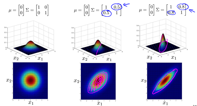
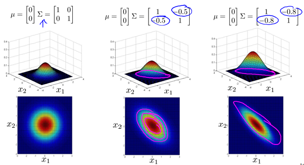
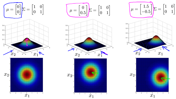
Anomaly detection using the multivariate Gaussian distribution

Multivariate Gaussian(Normal) distribution

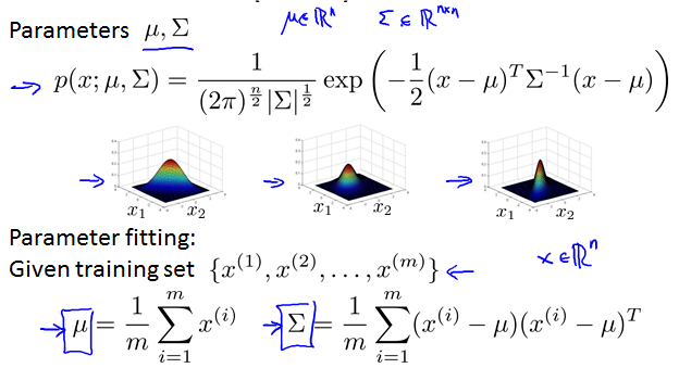
Anomaly detectioin with the multivariate Gaussian

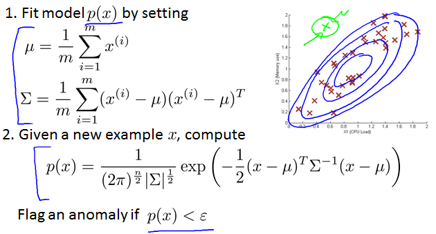
Relationship to original model

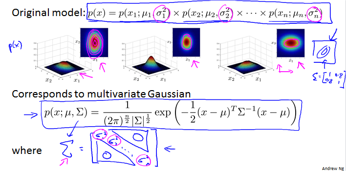
original model对应只有$\Sigma$主对角线有值的multivariate Gaussian。

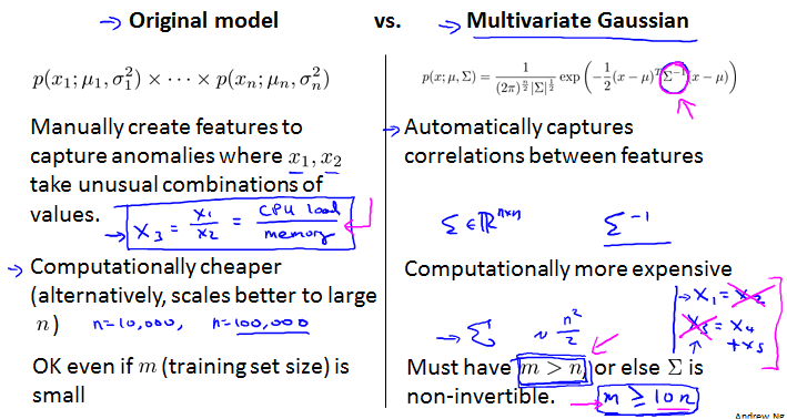
Recommender Systems

Problem formulation

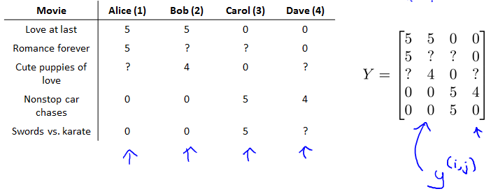
Example: Predicting movie ratings

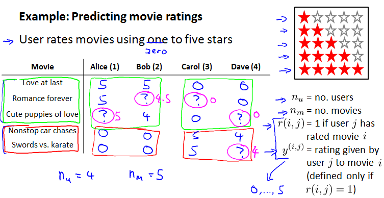
feature很重要。

Content-based recommendations

之所以叫这个名字是因为我们知道features of the content，比如movie有多romance多action。
Content-based recommender systems

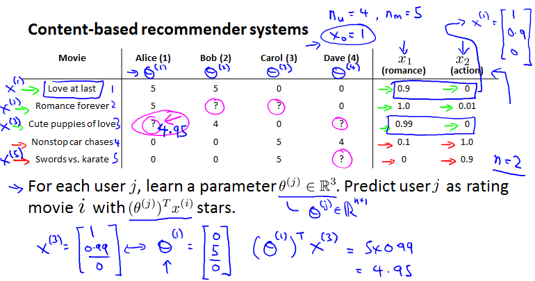
$n_u$是User数，$n_m$是Movie数。按惯例添加feature之$x_0=1$。下面的例子是预测Alice对Cute puppies of love的预测。

Problem formulation

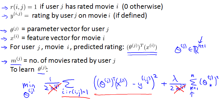
是一个linear regression problem.

Optimization objective:

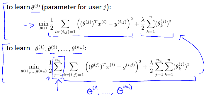
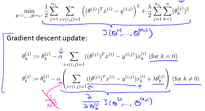
Optimization algorithm:

Collaborative filtering

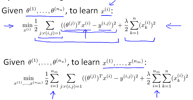
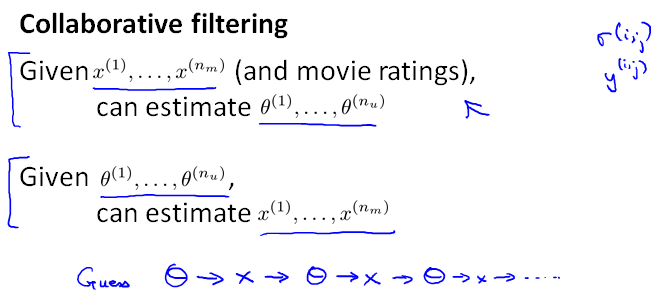
这种不需要知道features of content。它会feature learning。每个用户都让算法的表现更好一点，所以叫Collaborative。
Problem motivation

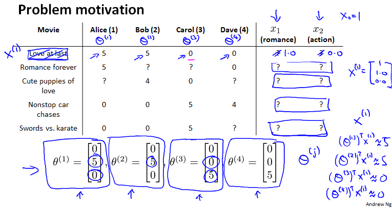
每个用户告诉我们她们对各种电影的喜好，就是$\theta$。${\theta}_0$都是0.

Optimization algorithm

Collaborative filtering

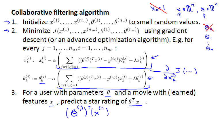
Collaborative filtering algorithm

Collaborative filtering optimization objective

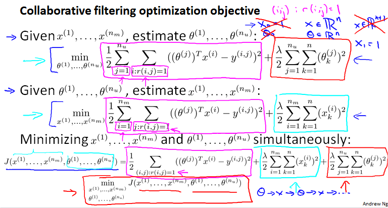
Collaborative filtering algorithm

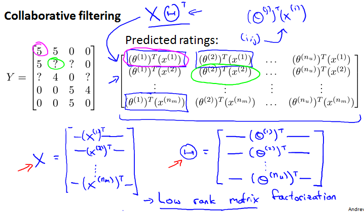
Vectorization: Low rank matrix factorization

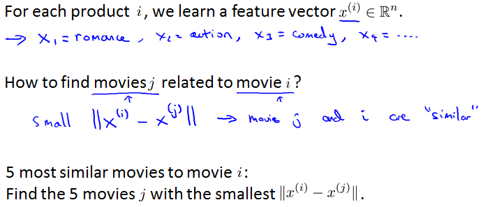
Finding related movies

Implementational detail: Mean normalization

Users who have not rated any movies

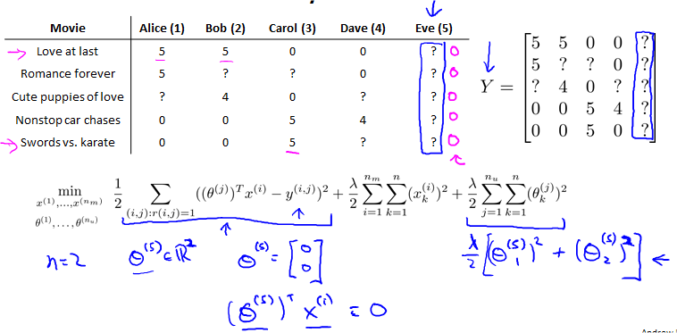
只有最后一部分会起效果，而对其最小化，$\theta$$就全是0，预测也就全是0。这样就不是太好。可以推荐一些平均值评价高的，使用mean normalization。

Mean Normalization:

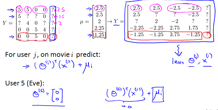
Large Scale Machine Learning

Learning with large datasets

Machine learning and data
之前见过这个例子。It’s not who has the best algorithm that wins. It’s who has the most data.

Learning with large datasets

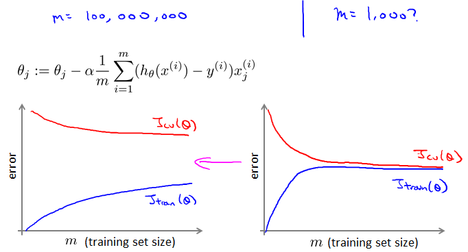
这样一步就要计算m次求和。

Stochastic gradient descent

Linear regression with gradient descent

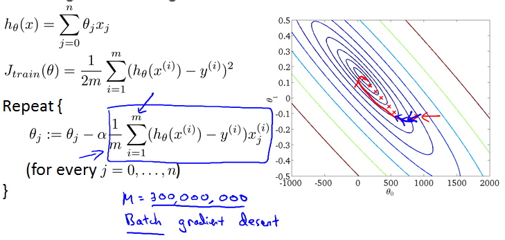
复习一下。数据很大时，这种gradient descent被叫做Batch gradient descent。
以linear regression为例，也适用于其他algorithms that are based on training gradient descent on a specific training set, like logistic regression, neural networks, etc.

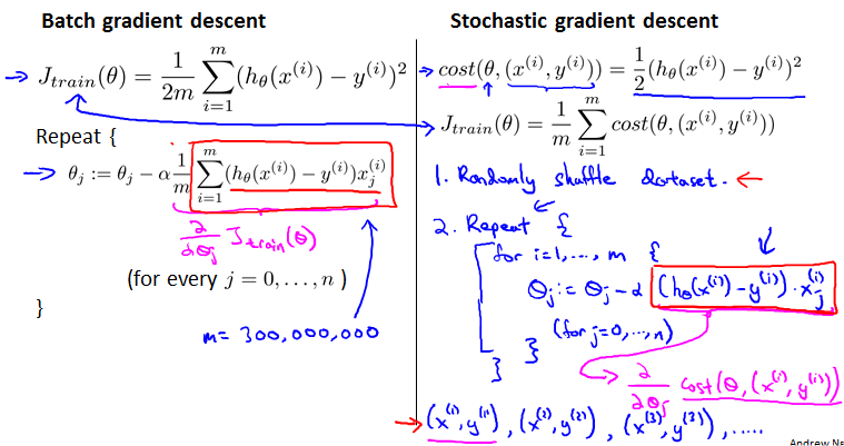
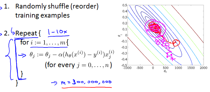
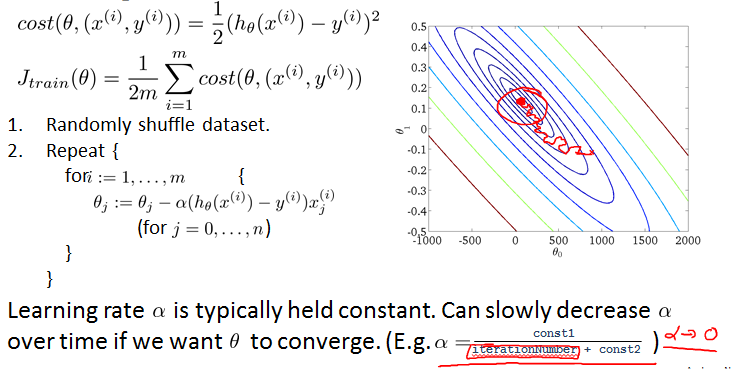
不再求和。随机排序，每次就看一个example。

Stochastic gradient descnet

Mini-batch gradient descent

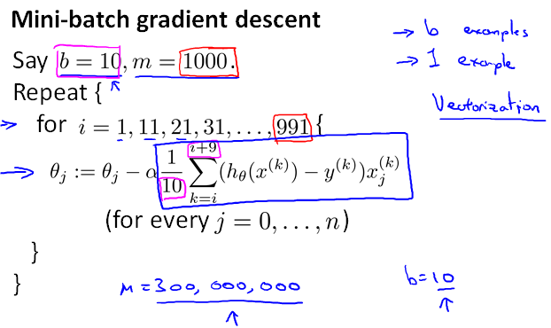
Mini-batch gradient descent
Batch gradient descent: Use all m examples in each iteration.
Stochastic gradient descent: Use 1 example in each iteration.
Mini-batch gradient descent: Use b examples in each iteration.

Stochastic gradient descent convergence

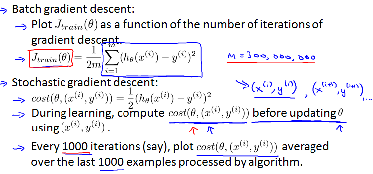
Checking for convergence


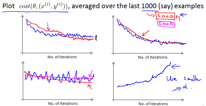
$\alpha$小一点，抖动会小一点，曲线更平滑。
如果每5000而不是每1000画一次，曲线更平滑。
如果cost曲线在上升，使用小一点的$\alpha$。

Stochastic gradient descent

Online learning

Online learning

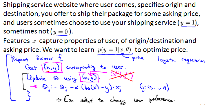
x是起始位置、我们开的价格等feature。y是1或0表示顾客是否使用我们的shipping service。每次只看一个顾客。

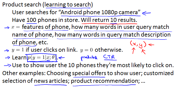
Other online learning example:

Map-reduce and data parallelism

Map-reduce

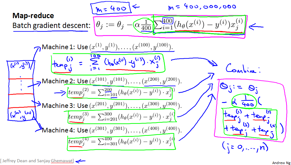
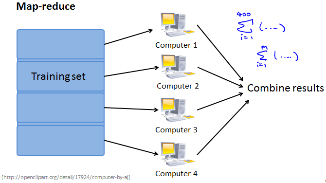
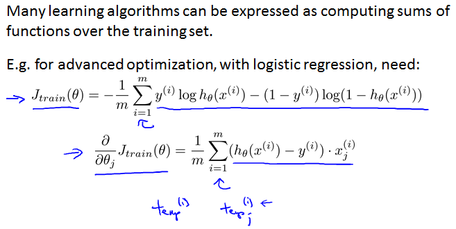
Map-reduce and summation over the training set

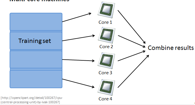
Multi-core machines

Application Example Photo OCR

Problem description and pipeline

The Photo OCR problem

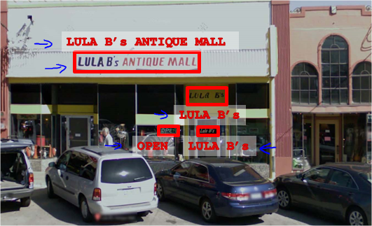
Photo Optical Character Recognition.

Photo OCR pipeline


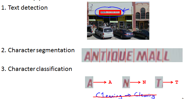
每一个部分有1-5个engineer。

Sliding windows

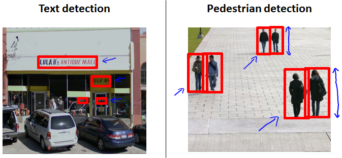
因为图片中的文字区域aspect ratio可能不同，行人识别要比其容易一些。

Supervised learning for pedestrian detection

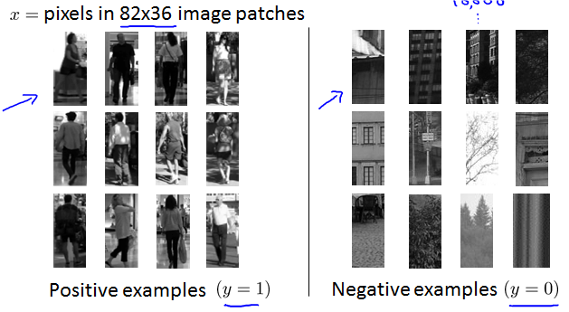
Sliding window detection

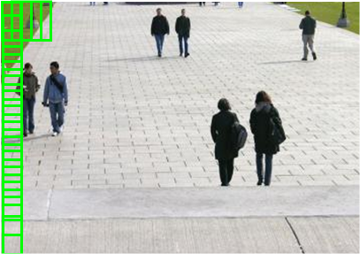
定义一个window，然后一点点移动，寻找行人。移动的距离叫做step-size/stride。

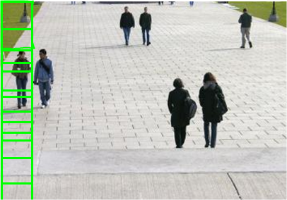
逐渐用更大一点的window。这个window在处理时也会缩小为82*36.

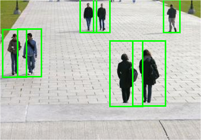
直到找到所有行人。

Text detection


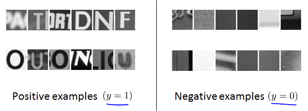
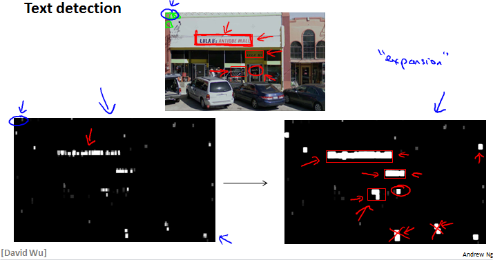
白色区域是算法认为的文字处，灰色是疑似处。然后进行expansion。去掉aspect radio不对劲的，比如垂直细长条。

1D Sliding window for character segmentation

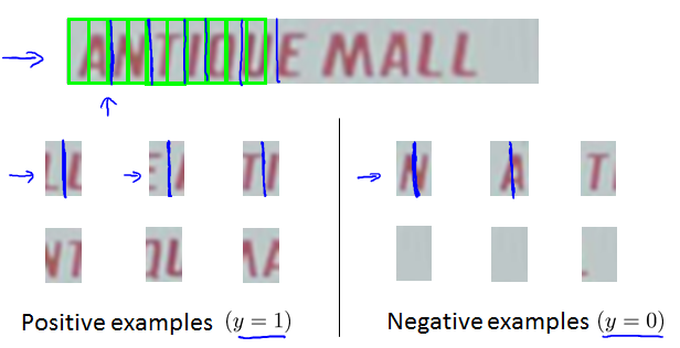
图中间是否有一个空白patch。

Getting lots of data: Artificial data synthesis

Character recognition

Artificial data synthesis for photo OCR


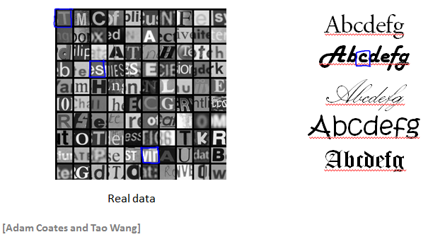
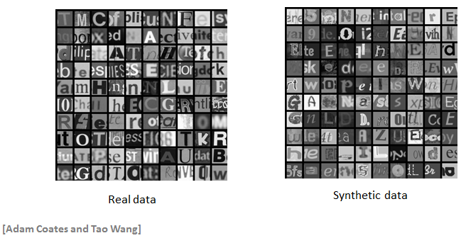
想要更多更多training set，找字体库，粘贴到随机背景上。这种方法是无中生有。

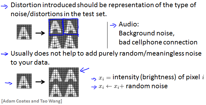
Synthesizing data by introducing distortions

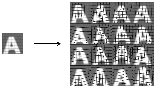
将原有字体变形。这种方法是从小样本生产大样本。

或者声音的例子：

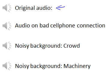
Discussion on getting more data

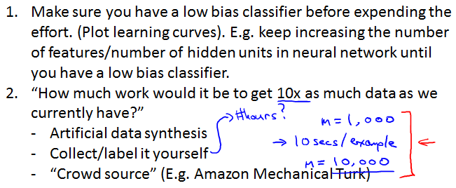
A sanity check with learning curves, that having more data would help. Ask yourself seriously: what it takes to get ten times much creative data as you currently have, and not always, but sometimes, you may be surprised by how easy that turns out to be.

Ceiling analysis: What part of the pipeline to work on next

不要浪费时间，事先估算每阶段工作量，安排好时间。
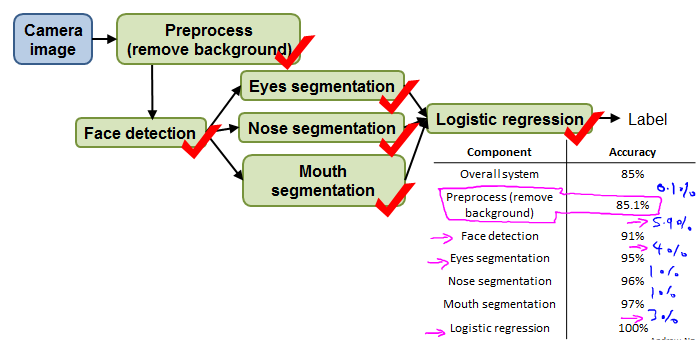
Estimating the errors due to each component(ceiling analysis)

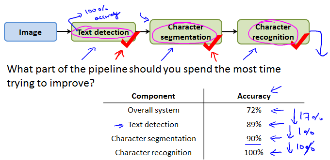
除了待测定的阶段，手动给每一个之前的阶段正确答案，然后看看总体系统的accuracy如何，这样就大概知道每个阶段大概需要做多少工作。

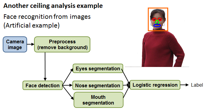
Another ceiling analysis example

Conclusion

Summary and Thank you

---

(¦3[▓▓]  好开心!