Model Evaluating 模型评估与选择
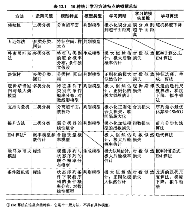
模型种类比较
No Free Lunch Theorem
Here is no method which outperforms all others for all tasks.
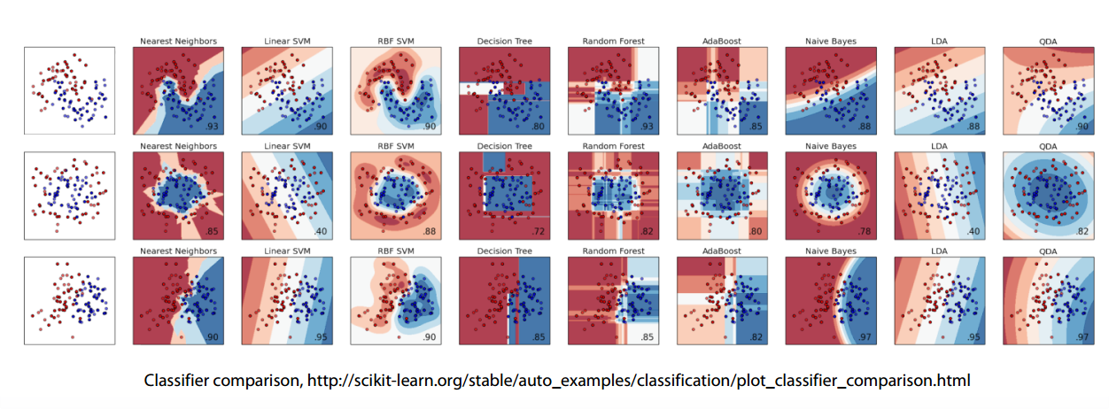
The most powerful methods are Gradient Boosted Decision Trees and Neural Networks.
But you shouldn’t underestimate the others
- Linear models split space into 2 subspaces.
- Tree-based methods splits space into boxes.
- k-NN methods heavily rely on how to measure points “closeness”.
- Feed-forward NNs produce smooth non-linear decision boundary.
经验误差与过拟合
训练时的误差是经验误差 empirical error;新样本上的误差是泛化误差 generalization error。我们需要泛化误差小的学习器。
overfitting / underfitting
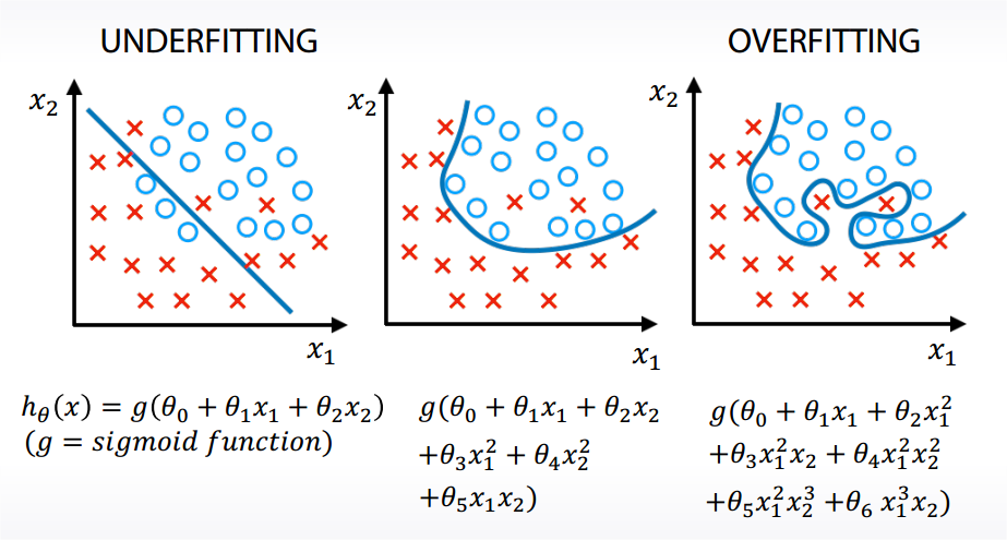
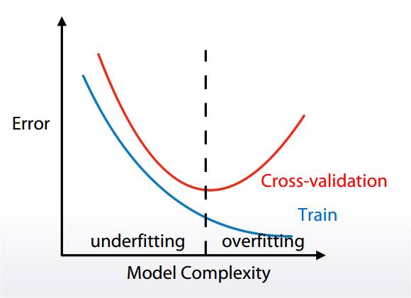
- Underfitting refers to not capturing enough patterns in the data.
- Generally, overfitting refers to.
a. capturing noize.
b. capturing patterns which do not generalize to test data.
评估方法
此处只考虑了泛化误差,现实任务中往往还会考虑时间开销、存储开销、可解释性等方面的因素。
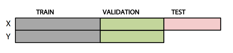
基于验证集 Validation Set 来进行模型选择和调参。
方法
- Holdout 留出法
- Cross Validation 交叉验证法
- K-fold
- Leave-one-out 留一法
- Bootstrapping 自助法
- Parameter Tuning 调参
Causes of validation problems:
- Too little data.
- Too diverse and inconsistent data.
- Incorrect train/test split.
- Different distributions in train and test.
- Overfitting.
Holdout 留出法
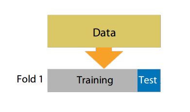
Holdout: ngroups = 1
sklearn.model_selection.ShuffleSplit
分割数据集时可能有多种方法:
- Random, rowwise
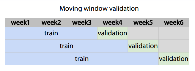
- Timewise - Moving window
- By id
Cross Validation 交叉验证法
K-fold
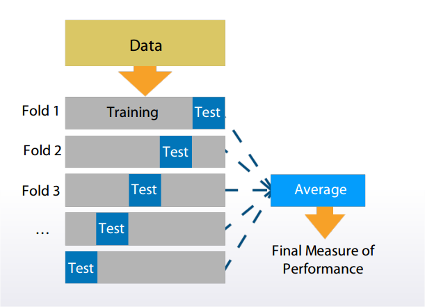
K-fold: ngroups = k
sklearn.model_selection.Kfold
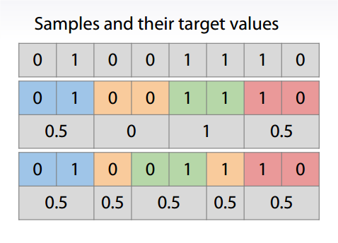
需要注意的是,training set 和 test set 应该尽可能保持数据分布的一致性。如果从采样 sampling 的角度来看待数据集的划分过程,则保留类别比例的采样方式通常称为分层采样 stratification sampling。
Stratification preserve the same target distribution over different folds.
Stratification is useful for:
- Small datasets.
- Unbalanced datasets.
- Multiclass classification.
Leave-one-out
特例,test set 里只有一个样本。
优点:training set 与实际使用的类似,可能比其他方式更准确。
缺点:在数据集比较大时,开销很大。
Bootstrapping 自助法
为了减少训练样本规模不同造成的影响,同时还能比较高效地进行实验估计。
以自助采样方式 bootstrap sampling 为基础:每次随机从初始训练集中挑选一个样本,将其拷贝放入训练集,然后再将该样本放回初始训练集中,使得该样本在下次采样时仍有可能被采到;重复m次。
做一个简单的估计,样本在m次采样中始终不被采到的概率为,取极限得到0.368,即约有36.8%的样本未出现在采样数据集中。
自助法在数据集较小,难以有效划分训练/测试集时很有用。对集成学习也有好处。但改变了初始数据集的分布,可能有估计误差。所以如果数据集够用就不用此方法。
Parameter Tuning 调参
对每个参数选定一个范围和变化步长,然后从候选值中产生选定值进行训练。选择太多,调参工作量很大。
性能度量 Metrics
Chosen metric determines optimal decision boundary.
- Regression
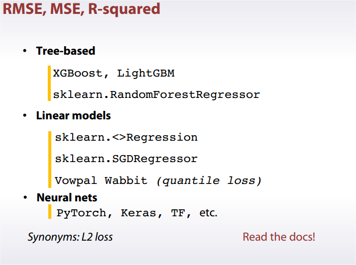
MSE, RMSE, R-squared
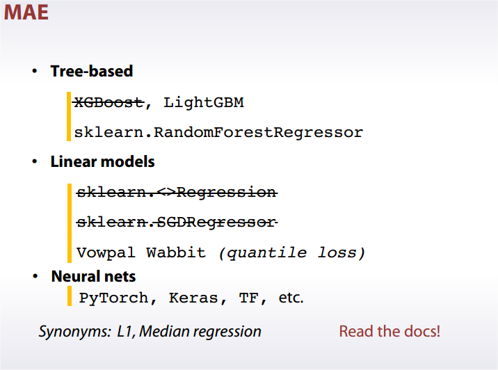
MAE
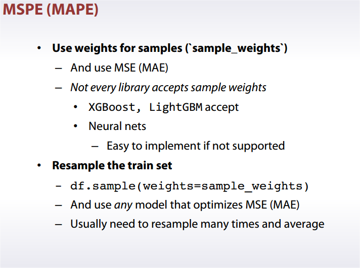
®MSPE, MAPE
®MSLE - Classification:
Accuracy, LogLoss, AUC, Confusion Matrix, Precision, Recall, F1 Score
Cohen’s (Quadratic weighted) Kappa
代价敏感错误率与代价曲线
注意 Loss 和 Metric 的区别:
- Target metric is what we want to optimize.
- Optimization loss is what model optimizes.
Regression metrics
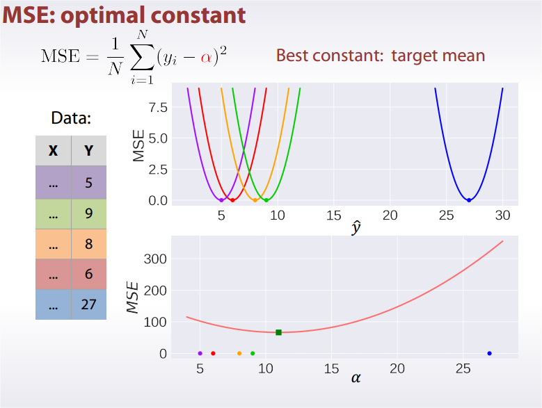
MSE: Mean Square Error
Best constant for is target mean.
TMSE: Root Mean Square Error
R-squared
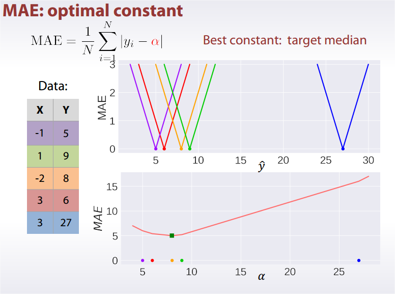
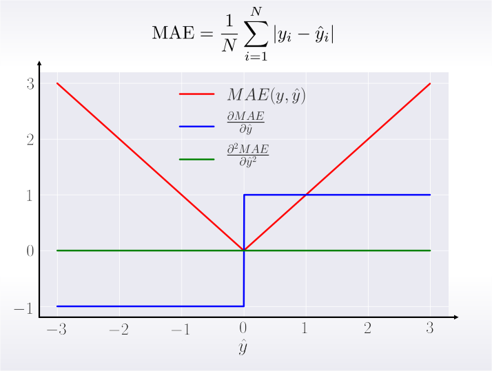
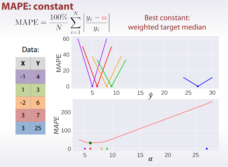
MAE: Mean Absolute Error
Best constant for is target median.
Derivatives:
From MSE and MAE to MSPE and MAPE
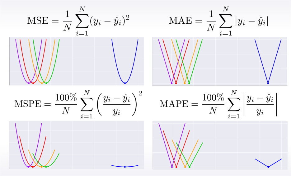
MSPE, MAPE
Best constant: weighted target mean.
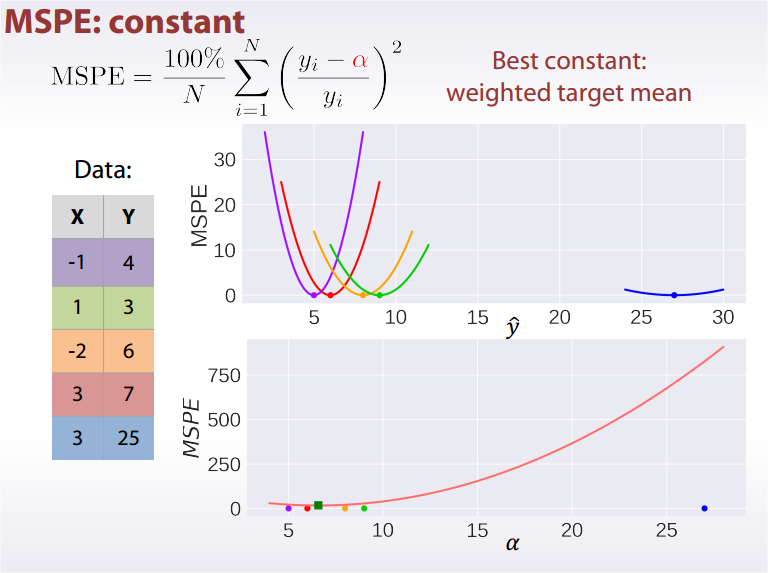
Best constant: weighted target mean.
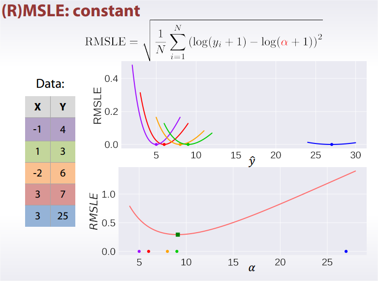
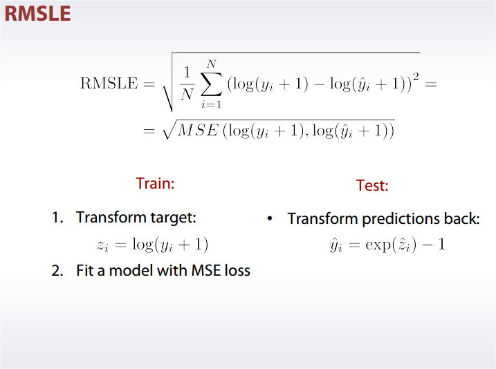
®MSLE: Root Mean Square Logarithmic Error
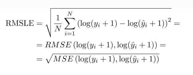
Best constant in log space is mean target value, exponentiate it to get an answer.
Comparison
比较
- MSE, RMSE, R-squared
They are the same from optimization perspective. - MAE
Robust to outliers. - ®MSPE
Weighted version of MSE. - MAPE
Weighted version of MAE. - ®MSLE
MSE in log space.
MAE vs. MSE
- Do you have outliers in the data?
Use MAE. - Are you sure they are outliers?
Use MAE. - Or they are just unexpected values we should still care about?
Use MSE.
To Optimize
Classification Metrics
Accuracy Score
How frequently our class prediction is correct.
Best constant: predict the most frequent class.
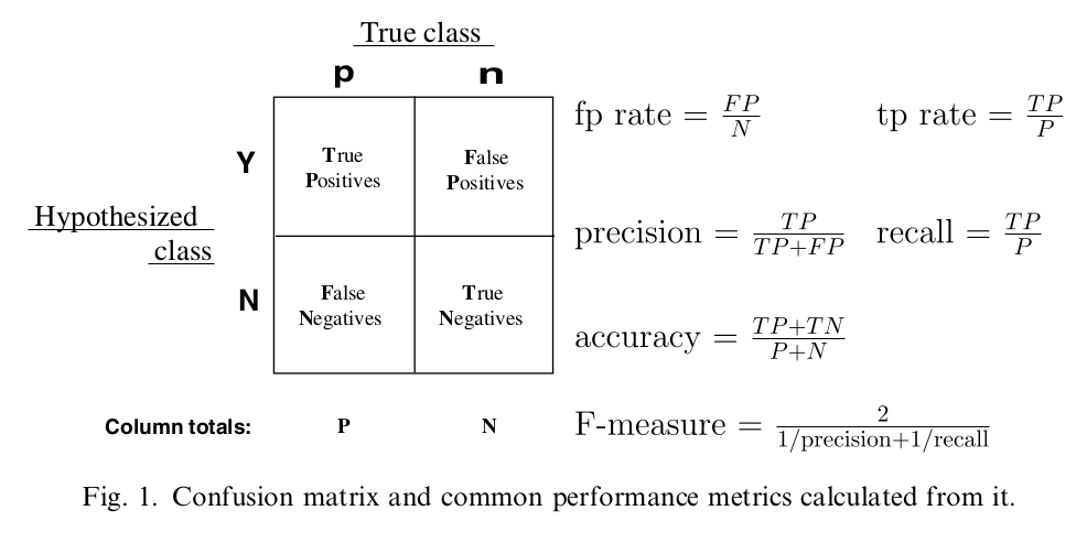
Confusion Matrix, Precision, Recall, F1 Score
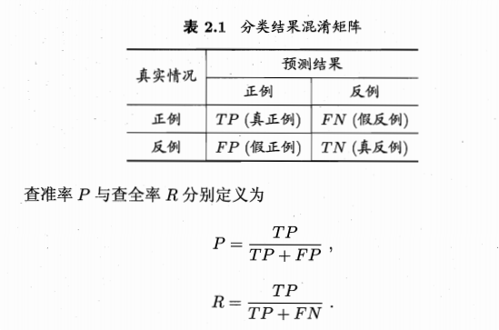
Precision,查准率,所有预测为 true 的里面有多少是正确的。
Recall,查全率,所有真正为 true 的里面有多少我预测到了。
Precision 和 Recall 是一对矛盾的度量。为了调和,引入 F1 Score。
即
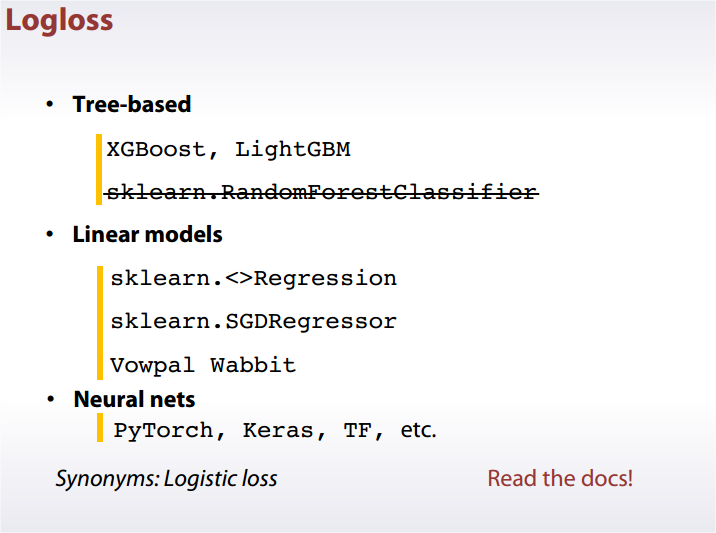
Logarithmic Loss (logloss)
Binary
Multiclass
In practice
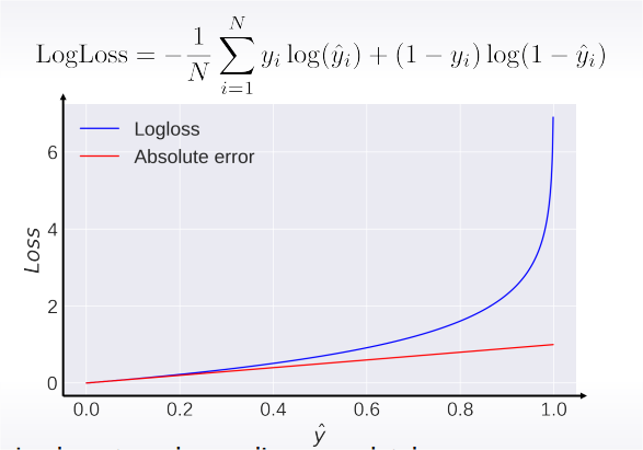
Logloss strongly penalizes completely wrong answers.
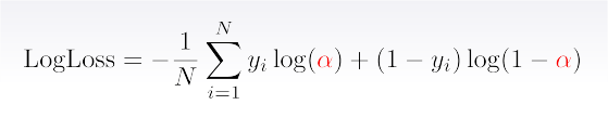
Best constant: set to frequency of -th class.
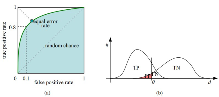
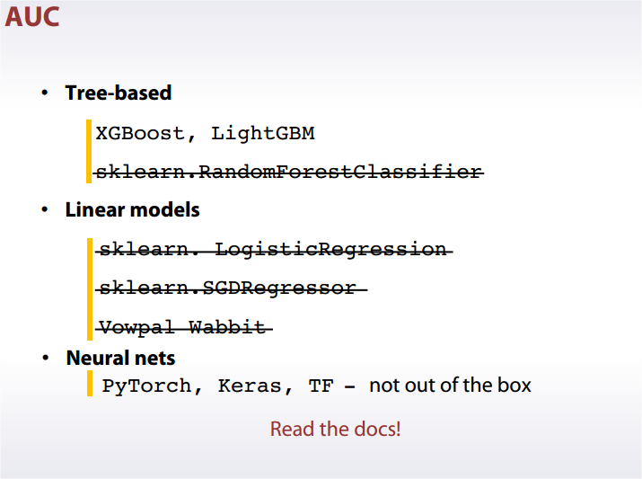
Area Under Curve (AUC ROC)
ROC(Receiver Operating Characteristic)曲线和AUC常被用来评价一个二值分类器(binary classifier)的优劣。横坐标为false positive rate(FPR),纵坐标为true positive rate(TPR)。
接下来我们考虑ROC曲线图中的四个点和一条线。第一个点,(0,1),即FPR=0, TPR=1,这意味着FN(false negative)=0,并且FP(false positive)=0。Wow,这是一个完美的分类器,它将所有的样本都正确分类。第二个点,(1,0),即FPR=1,TPR=0,类似地分析可以发现这是一个最糟糕的分类器,因为它成功避开了所有的正确答案。第三个点,(0,0),即FPR=TPR=0,即FP(false positive)=TP(true positive)=0,可以发现该分类器预测所有的样本都为负样本(negative)。类似的,第四个点(1,1),分类器实际上预测所有的样本都为正样本。经过以上的分析,我们可以断言,ROC曲线越接近左上角,该分类器的性能越好。
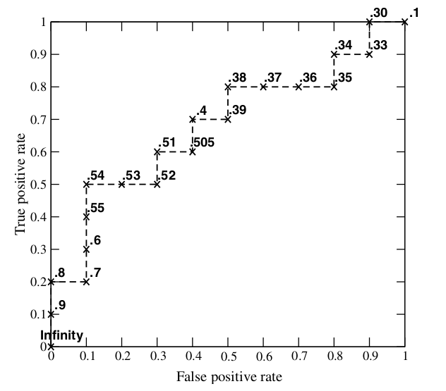
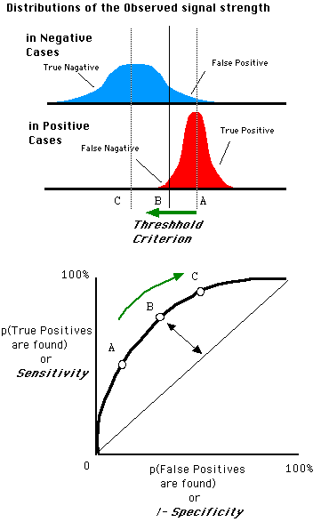
ROC 曲线生成过程:根据每个测试样本属于正样本的概率值 Score从大到小排序。接下来,我们从高到低,依次将 Score 值作为阈值threshold,当测试样本属于正样本的概率大于或等于这个threshold时,我们认为它为正样本,否则为负样本。每次选取一个不同的threshold,我们就可以得到一组FPR和TPR,即ROC曲线上的一点。迭代。
AUC (Area Under Curve) 为 ROC 曲线下的面积。使用AUC值作为评价标准是因为很多时候ROC曲线并不能清晰的说明哪个分类器的效果更好,而作为一个数值,对应AUC更大的分类器效果更好。
Random predictions lead to AUC = 0.5
ROC的优点:当测试集中的正负样本的分布变化的时候,ROC曲线能够保持不变。
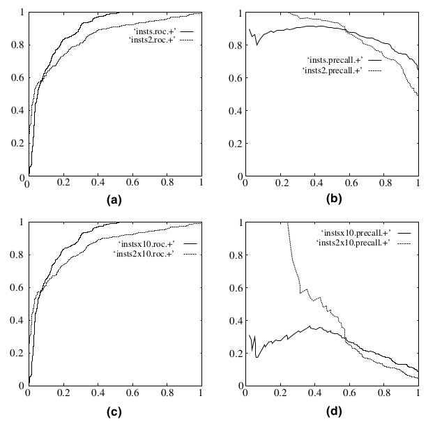
在上图中,(a)和©为ROC曲线,(b)和(d)为Precision-Recall曲线。(a)和(b)展示的是分类其在原始测试集(正负样本分布平衡)的结果,©和(d)是将测试集中负样本的数量增加到原来的10倍后,分类器的结果。可以明显的看出,ROC曲线基本保持原貌,而Precision-Recall曲线则变化较大。
Cohen’s Kappa
todo ref[5]
代价敏感错误率与代价曲线
现实任务中,常有不同类型的错误所造成的后果不同的情况。非均等代价。
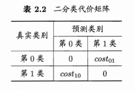
将原来公式中只计算错误次数的地方,都乘以对应的 cost。
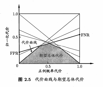
ROC 曲线也不再适用于此场合,应该用代价曲线 cost curve。
To Optimize
比较检验
使用某种实验评估方法测得学习器的某个性能度量结果,然后进行比较。这个比较并不只是单纯比较两个数的大小就可以了。原因:
- 需要比较泛化性能,而实验评估的结果是测试集上的性能,两者未必相同。
- 测试集上的性能与测试集本身有很大关系,大小不同的测试集、样例不同的测试集,都有影响。
- 很多机器学习算法本身有一定随机性,即使用相同参数在同一个测试集上多次运行,结果也不一定相同。
这时就要用到统计假设检验 hypothesis test。基于假设检验结果我们可以推断出,若在测试集上观察到学习器A比B好,则A的泛化性能是否在统计意义上优于B,以及这个结论的把握有多大。
本节默认以错误率为性能度量,记为。
假设检验
交叉验证t检验
McNemar 检验
Friedman 检验与 Nemenyi 后续检验
偏差与方差
Ref
[1] Coursera - How to Win a Data Science Competition
[2] 机器学习 - 周志华
[3] 统计学习方法
[4] https://www.jianshu.com/p/c61ae11cc5f6
[5] http://www.pmean.com/definitions/kappa.htm