Gradient Boosting Decision Tree

A Stellar Hiker

2018-05-13

Gradient Boosting Decision Tree (GBDT) (一般用 CART)是一种常用来分类、回归的模型，而 XGBoost 与 LightGBM 是基于 GBDT 的两种实现。
GDBT 是一种使用 gradient 作为信息，将不同的弱分类 Decision Tree 进行加权，从而获得较好性能的方法。

GBDT

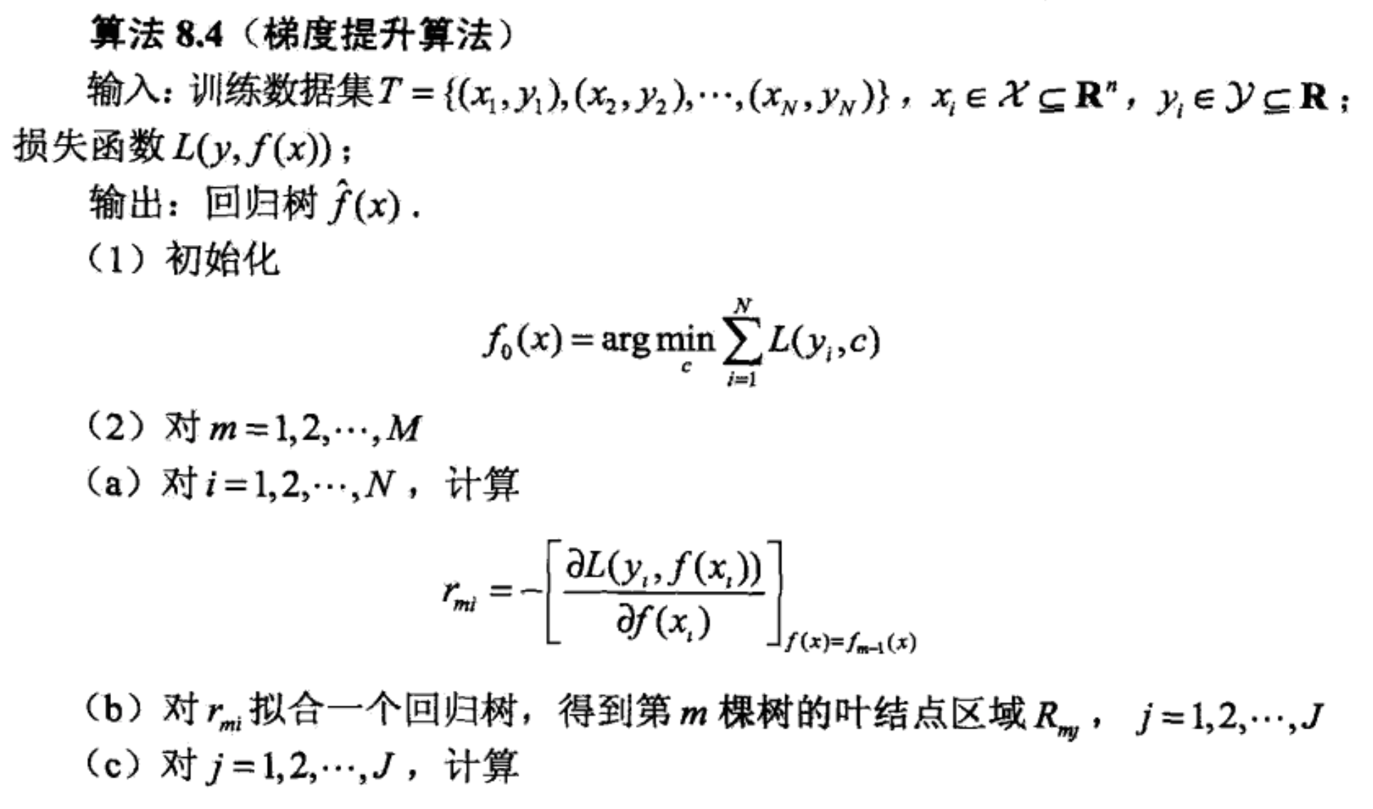
当损失函数是一般损失函数时，使用 gradient boosting 算法。这是利用最速下降法的近似方法，其关键是利用损失函数的负梯度在当前模型的值(下式 a)作为回归问题提升树算法中的残差的近似值，拟合一个回归树。
Image Loading

换一种写法 (我觉得更好理解)。
步骤：

初始化。
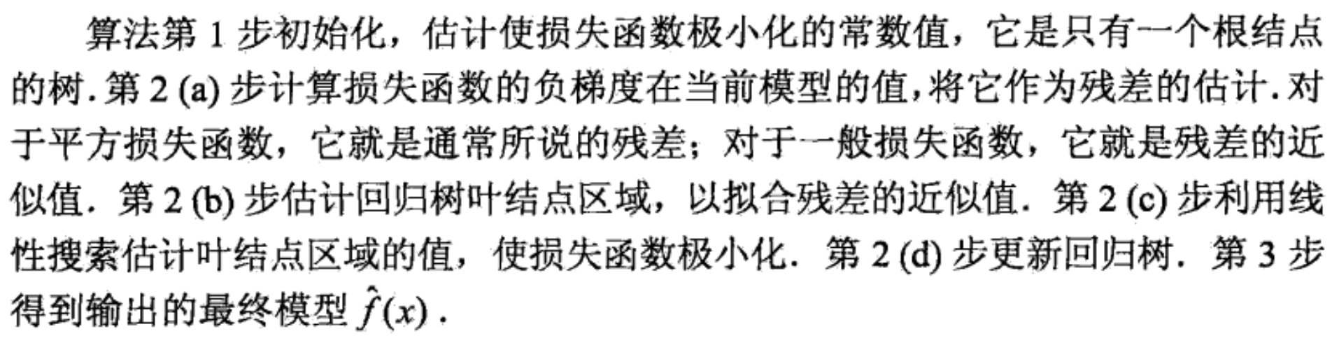
初始化 $\hat y$ 在第0时刻的值。取使损失函数极小化的常数值。
求残差，通过负梯度拟合。

$g_i = - \frac{\partial Loss(y_i, \hat y^{(t-1)})}{\partial \hat y^{(t-1)}}$

构建决策树，拟合残差。得到第 t 个决策树 $f_t$ 。
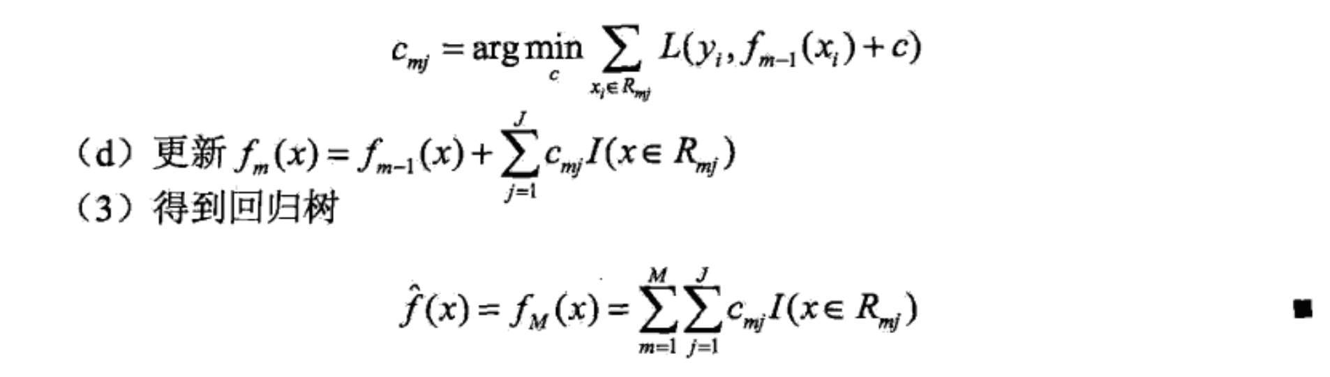
求叶节点权重。
树 $k$ 的第 $j$ 个叶节点：

w_{kj} = \arg \min_w \sum_{x_i \in 叶} Loss(y_i, y_i^{(t-1)} + w)

更新输出 $y$ 。

$y(t) = y(t-1) + \alpha f_t$

XGBoost

eXtreme Gradient Boosting。
作者的 PPT：
(如果尺寸有问题缩放再重置一下。)

Theory

Model

$\hat y_i = \sum_{k=1}^K f_k(x_i), f_k \in \mathcal{F}$

$f_t(x) = w_{q(x)}, w \in R^T, q: R^d \rightarrow \{1,2, \ldots, T\}$

其中 $w$ 是 The leaf weight of the tree，叶节点的权重。 $q$ 是 The structure of the tree，走到叶节点的所有分支，也即树结构。

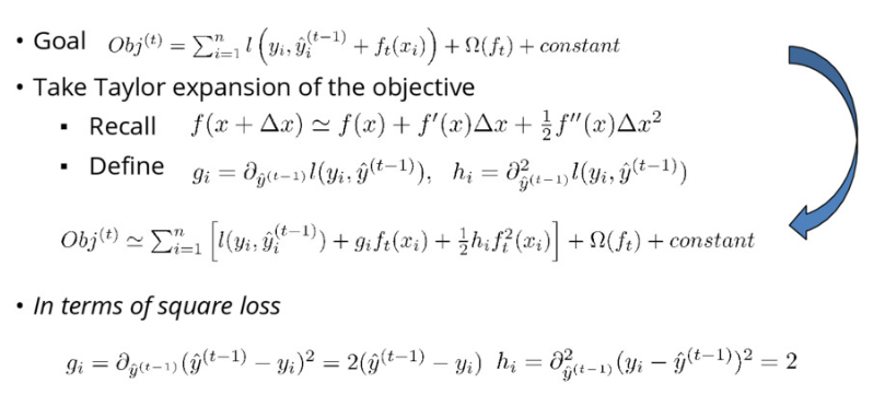
Objective

$Obj = \sum_{i=1}^n l(y_i, \hat y_i) + \sum_{k=1}^K \Omega(f_k)$

$\Omega(f_k) = \gamma T + \frac{1}{2} \lambda \sum_{j=1}^T w^2_j$

其中 Obj 的第一部分是 Training Loss，measures how well model fit on training data。第二部分是 Regularization，measures complexity of trees。
具体到正则项的表示， $T$ 表示 Number of leaves，后半部分的非常数部分表示 L2 norm of leaf scores。
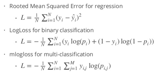
而这里的 Loss 可以选择多种，如下图三种可分别用于回归，二分类，多分类。
Loss Function

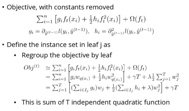
New Objective

先用泰勒展开估计，Taylor Expansion Approximation of Loss。

去掉常数，再把维度从样本数变成叶子数。因为属于同一个叶子节点的样本数的 weight 是相同的。
New Objective

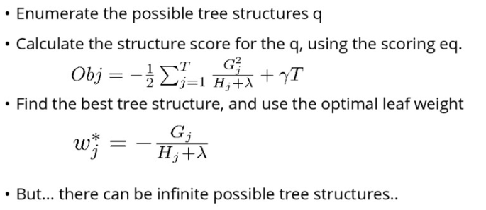
Single Tree Generation

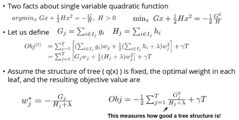
The Structure Score
假设树结构已经固定，Obj 对 w 求导，求出最优 w，再代回到 Obj，就是 Structure Score。越小说明树越好。

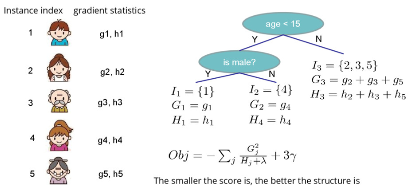
The Structure Score Calculation
一个计算的例子。

Searching Algorithm for Single Tree
全部遍历不现实。

Greedy Learning of the Tree
用 Greedy 方式。

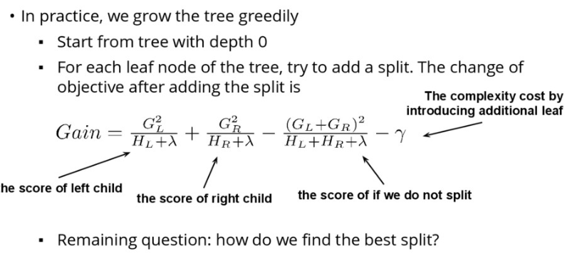
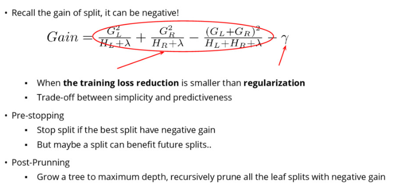
Pruning and Regularization
注意这个正则项，如果得不偿失就要剪枝。

使用

Code Example

Classification

# First XGBoost model for Pima Indians dataset
from numpy import loadtxt
from xgboost import XGBClassifier
from sklearn.model_selection import train_test_split
from sklearn.metrics import accuracy_score
# load data
dataset = loadtxt('pima-indians-diabetes.csv', delimiter=",")
# split data into X and y
X = dataset[:,0:8]
Y = dataset[:,8]
# split data into train and test sets
seed = 7
test_size = 0.33
X_train, X_test, y_train, y_test = train_test_split(X, Y, test_size=test_size, random_state=seed)
# fit model no training data
model = XGBClassifier()
model.fit(X_train, y_train)
# make predictions for test data
y_pred = model.predict(X_test)
predictions = [round(value) for value in y_pred]
# evaluate predictions
accuracy = accuracy_score(y_test, predictions)
print("Accuracy: %.2f%%" % (accuracy * 100.0))

Using XGBoost in Pipelines

import pandas as pd
import xgboost as xgb
import numpy as np
from sklearn.preprocessing import StandardScaler
from sklearn.pipeline import Pipeline
from sklearn.model_selection import cross_val_score

names = ['crime', 'zone', 'industry', 'charles', 'no', 'rooms', 'age']
data = pd.read_csv('boston_housing.csv', names = names)
X, y = data.iloc[:,:-1], data.iloc[:,-1]

xgb_pipeline = Pipeline[('st_scaler', StandardScaler()), ('xgb_model', xgb.XGBRegressor())]
scores = cross_val_score(xgb_pipeline, X, y, scoring = 'neg_mean_squared_error', cv = 10)

final_avg_rmse = np.mean(np.sqrt(np.abs(scores)))
print('Final XGB RMSE:', final_avg_rmse)

Tuning XGBoost Hyperparameters

import pandas as pd
import xgboost as xgb
import numpy as np
from sklearn.preprocessing import StandardScaler
from sklearn.pipeline import Pipeline
from sklearn.model_selection import RandomizedSearchCV

names = ['crime', 'zone', 'industry', 'charles', 'no', 'rooms', 'age']
data = pd.read_csv('boston_housing.csv', names = names)
X, y = data.iloc[:,:-1], data.iloc[:,-1]
xgb_pipeline = Pipeline[('st_scaler', StandardScaler()), ('xgb_model', xgb.XGBRegressor())]

gbm_param_grid = {
    'xgb_model__subsample': np.arange(.05, 1, .05),
    'xgb_model__max_depth': np.arange(3, 20, 1),
    'xgb_model__colsample_bytree': np.arange(.1, 1.05, .05)
}

randomized_neg_mse = RandomizedSearchCV(estimator = xgb_pipeline,
    param_distributions = gbm_param_grid, n_iter = 10,
    scoring = 'neg_mean_squared_error', cv = 4)

randomized_neg_mse.fit(X, y)

print('Best rmse: ', np.sqrt(np.abs(randomized_neg_mse.best_score)))
print('Best model: ', randomized_neg_mse.best_estimator_)

Parameters

见文档 https://github.com/dmlc/xgboost/blob/master/doc/parameter.rst 。

Control Overfitting

Control the model complexity
max_depth, min_child_weight, gamma
Robust to noiss
subsample, colsample_bytree

Deal with Imbalanced Data

Only care about the ranking order
Balance the positive and negative weights, by scale_pos_weight.
Use “auc” as the evaluation metric.
Care about predicting the right probability
Cannot re-balance the dataset.
Set parameter max_delta_step to a finite number (say 1) will help convergence.

特点

变化1：提高了精度 - 对Loss的近似从一阶到二阶
传统GBDT只使用了一阶导数对loss进行近似，而XGBoost对Loss进行泰勒展开，取一阶导数和二阶导数。同时，XGBoost的Loss考虑了正则化项，包含了对复杂模型的惩罚，比如叶节点的个数、树的深度等等。
通过对Loss的推导，得到了构建树时不同树的score。具体score计算方法见论文Sec 2.2。
变化2：提高了效率 - 近似算法加快树的构建
XGBoost支持几种构建树的方法。
第一：使用贪心算法，分层添加decision tree的叶节点。对每个叶节点，对每个feature的所有instance值进行排序，得到所有可能的split。选择score最大的split，作为当前节点。
第二：使用quantile对每个feature的所有instance值进行分bin，将数据离散化。
第三：使用histogram对每个feature的所有instance值进行分bin，将数据离散化。
变化3：提高了效率 - 并行化与cache access
XGBoost在系统上设计了一些方便并行计算的数据存储方法，同时也对cache access进行了优化。这些设计使XGBoost的运算表现在传统GBDT系统上得到了很大提升。

LightGBM

todo

LightGBM目前是XGBoost的有力竞争对手。就目前的一些report来说，LightGBM在更大、更sparse的数据上，比XGBoost的速度提升10倍有余；而它的精确度却没有很显著的损失。

变化1：让训练样本更少
因为GBDT可以看做对残差大的样本加权更大（因为下一个决策树是用来拟合上一个决策树之后的残差的），所以对残差小的样本，LightGBM认为它们对树的学习不是很重要，所以对这部分样本进行了采样。
变化2：让特征更少
因为很多数据集的feature是非常sparse的，所以会有很多互斥的features。互斥的features指两个features内积基本为0。
LightGBM将这些互斥的feature相加，得到了更少的feature bundles。得到最少feature bundles是一个np-hard的问题，LightGBM对这个问题也做了一些优化。

基于这两方面的improvements，LightGBM是目前来说表现最好的GBDT系统。

Ref

[1] 统计学习方法
[2] http://liangchen.soy/cn/GBDT/
[3] https://machinelearningmastery.com/gentle-introduction-xgboost-applied-machine-learning/
[4] http://datascience.la/xgboost-workshop-and-meetup-talk-with-tianqi-chen/
[5] https://xgboost.readthedocs.io/en/latest/
[6] https://github.com/dmlc/xgboost/tree/master/demo/guide-python
[7] https://www.datacamp.com/courses/extreme-gradient-boosting-with-xgboost
[8] https://machinelearningmastery.com/develop-first-xgboost-model-python-scikit-learn/